

| S+ | |
|
| S- |  |
 |
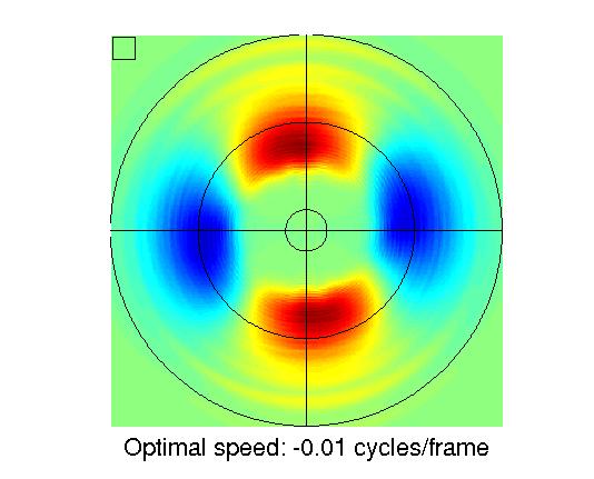
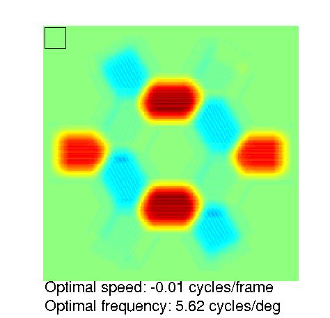
Using a two-dimensional Fourier analysis we extract from S+ several parameters that are used for example to generate the hexagonal test image (see below) or to make additional experiments with linear sine gratings. Here we report the orientation and frequency of the two components of S+ and the optimal speed, measured by the phase difference between S+ at time t and at time t+dt. The orientation is measured counterclockwise between 0 and 180 degrees, 0 being the horizontal direction. The frequency is reported in cycles/arc deg, assuming that an input patch is 0.5 arc deg large.
 |
 |
 |
 |
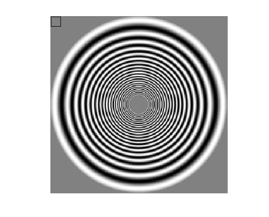
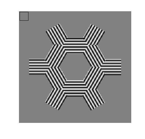
To study the response of the unit to a wide range of stimuli we use pairs of test images (one at time t and one at time t+dt). The response images are generated by scanning the test images, cutting at each point a 16x16 window, using it as an input to the unit, and plotting its output at the corresponding point. The black square in the upper left corner indicates the size of an input window.
In the analysis pages we show two different types of response images. They are generated using the test images shown above (second row). The left one consists of a circular pattern of sine waves with frequencies increasing from the circumference to the center. The ring patterns move outward with the preferred speed of the unit. This test image gives information not only about the whole range of frequencies and orientations to which the unit responds or by which it is inhibited, but also about the sensitivity to phase. If a unit is sensitive, the response image will show oscillations in the radial direction, while if there are no oscillations the unit is phase-invariant. Moreover, since at two opposite points of a ring the grating is moving in opposite directions, different responses indicate selectivity to the direction of motion. The right test image is used to investigate end- and width-inhibition. The hexagonal shape is oriented such that it is aligned with the preferred orientation of the considered unit. The gratings are tuned to the preferred frequency and move at the preferred speed of the unit. If a unit is selective for the length or width of the input, one notices a higher response at the borders of the hexagon, where only part of the input window is filled, than in the inner, where the whole input window is filled.
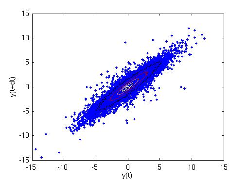
Beta value: 0.058
The beta value is the quantity optimized by SFA, and measures the temporal
variation of the output. It is here defined as
beta(y) = 1/(2*Pi) * sqrt(<dy/dt ^2>) .
In particular, a sine wave with period T has an beta value of 1/T.
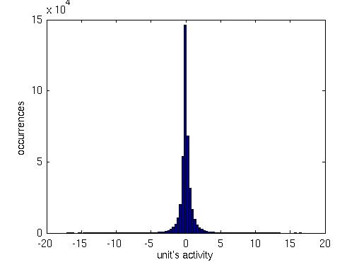
Kurtosis: 19.74
Kurtosis is the fourth moment of the distribution of the output
values. It is a measure of the sparseness of the unit, which is
considered to be a desirable property of a neural code according to
some efficiency arguments. We report it here to allow the comparison
with other theoretical models of V1 [1].
Sparseness: 67 %
This is another measure of the sparseness of the unit. It is defined as
Sparseness(y) = (1- (<abs(y)>^2/<y^2>)) / (1-(1/n))
This measure is normalized such that 100% correspond to a unit responding to
only one particular stimulus, while a unit scoring 0% responds to all
stimuli. We report it here to allow the comparison with experimental
studies [2].
 |
 |
[1] B. Willmore and D.J.Tolhurst. (2001).
Characterizing the sparseness of neural codes.
Network: Comput. Neural Syst. 12, 255-270
[2] W.E. Vinje and J.L. Gallant. (2000).
Sparse coding and decorrelation in primary visual cortex during natural vision.
Science, 287, 1273-1276