Bayesian Approaches
to Distribution Regression
Learning on Distributions, Functions, Graphs and Groups
NIPS 2017
Distribution regression
 -0.856
 0.562
0.562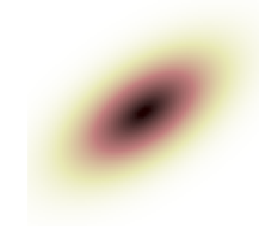
 1.39
1.39Labels Observe Model
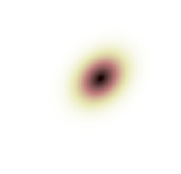
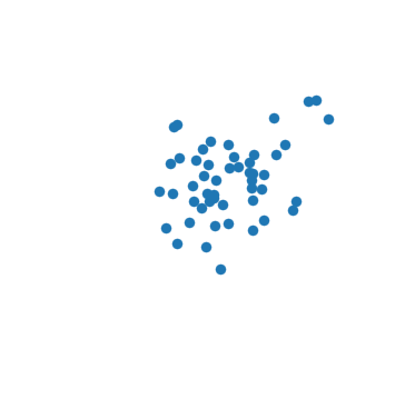
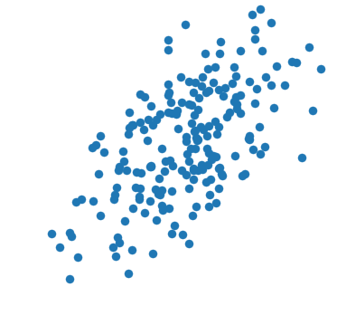
Different numbers of samples
Distribution regression applications
- “JIT” regression for EP messages [Jitkrittum+ UAI-15]
- Choose summary statistics for ABC [Mitrovic+ ICML-16]
- Infer demographic voting behavior [Flaxman+ KDD-15, 2016]
- Galaxy cluster mass from velocities [Ntampaka+ ApJ 2015/2016]
- Red shift estimation from galaxy clusters [Zaheer+ NIPS-17]
- Model radioactive isotope behavior [Jin+ NSS-16]
- Predict grape yields from vineyard images [Wang+ ICML-14]
- …
- (Plus lots of classification, anomaly detection, etc)
Distribution regression with kernel mean embeddings
- Standard approach [e.g. Muandet+ NIPS 2012]
- Choose RKHS with kernel
- e.g.
- Use mean embedding
- Reproducing property: for ,
- Mean embeddings are good representation for regression
Estimating kernel mean embeddings
- is a good summary of
- But don't know or ; just have samples
- Natural estimate: empirical mean
- Inner products:
- But…point estimate worse for small
Posterior for mean embeddings [Flaxman+ UAI 2016]
- Place prior:
- Likelihood is “observed” at points :
- Get a closed-form GP posterior for :
- Mean matches Stein shrinkage estimator [Muandet+ ICML 2014]
Distribution regression with kernel mean embeddings
- Model label as function of mean embedding:
- Estimate with ridge regression:
- Landmark approximation:
- Have uncertainty about both and
Shrinkage model
- Uses [Flaxman+ UAI 2016]'s GP posterior for
- Point estimate for weights
- Observations
- Landmark approximation:
- Get
- Can get MAP estimate for , , kernel params, …
Bayesian linear regression
- Assumes are known exactly: point estimate at
- Regression weight uncertainty:
- Observations:
- Posterior for is normal
- Hyperparameters: , , kernel params…
Full Bayesian Distribution Regression
- Shrinkage posterior for
- Normal model for regression weights:
- Observations
- is non-conjugate; MCMC inference with Stan
Models recap
| Model | Inference | ||
|---|---|---|---|
| Shrinkage | GP model | point est. | conjugate+MAP |
| BLR | point est. | normal | conjugate+MAP |
| BDR | GP model | normal | conjugate+MCMC |
Toy experiment
- Labels uniform over
- 5d data points:

have
Toy experiment: NLL
BDR shrinkage BLR in NLL:

Toy experiment results: MSE
Same BDR shrinkage BLR in MSE. (Predicting mean: 1.3)


Toy experiment
- Variant with constant , added noise:
- BDR BLR shrinkage in NLL, MSE
- BDR can take advantage of both situations
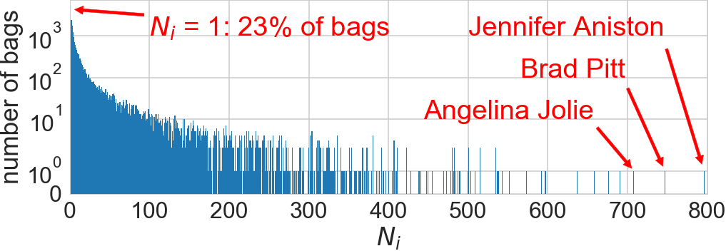
Age prediction from face images
 ,
,  ,
,  ,
, 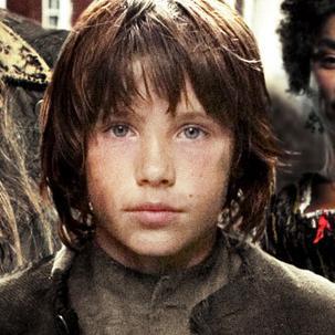 ,
, 
IMDb database [Rothe+ 2015]: 400k images of 20k celebrities
Age prediction results
Features: last hidden layer of Rothe et al.'s CNN

Shrinkage really helps!
Recap
Three Bayesian models for distribution regression:
| Model | Inference | ||
|---|---|---|---|
| Shrinkage | GP model | point est. | conjugate+MAP |
| BLR | point est. | normal | conjugate+MAP |
| BDR | GP model | normal | conjugate+MCMC |
- Both kinds of uncertainty can help
- BDR can take advantage of both settings
Bayesian Approaches to Distribution Regression
Ho Chung Leon Law, Dougal J. Sutherland, Dino Sejdinovic, Seth Flaxman