Efficient and principled score estimation
with kernel exponential families
arXiv:1705.08360
Our goal
- A multivariate density model that:
- Is flexible enough to model complex data (nonparametric)
- Is computationally efficient to estimate and evaluate
- Has statistical guarantees
Exponential families
- Can write many densities on as:
- Gaussian:
- Gamma:
- Density only sees data through (and )
- Can we make richer?
Infinitely many features with kernels!
- Kernel: “similarity” function
- e.g. exponentiated quadratic
- For any positive definite on , there's a reproducing kernel Hilbert space of functions on with
- is the infinite-dimensional feature map of

Functions in the RKHS
- Functions in are (closure of) linear combinations of :


Reproducing property
- Functions in are (closure of) linear combinations of :
- Reproducing property:
Kernel exponential families
- Lift parameters from to the RKHS , with kernel :
- Use and , so:
- Covers standard exponential families:
- e.g. normal distribution has
Rich class of densities
- For rich-enough that decay to 0,
is dense in the set of distributions that decay like- Examples of :
![]()
- Examples of :

Density estimation
- Given sample , want so that
- is hard to compute
- Maximum likelihood would need at each step: intractable
- Need a way to fit an unnormalized probabilistic model
- Could then estimate once after fitting
Unnormalized density / score estimation
- Don't necessarily need to compute afterwards
- (“energy”) lets us:
- Find modes (global or local)
- Sample (with MCMC)
- …
- The score, , lets us:
- Run HMC when we can't evaluate gradients
- Construct Monte Carlo control functionals
- …
- But again, need a way to find
Score matching in KEFs
- Idea: minimize Fisher divergence
- Under mild assumptions, integration by parts gives
- Estimate with
[Sriperumbudur, Fukumizu, Gretton, Hyvärinen, and Kumar, JMLR 2017]
Score matching in kernel exp. families
- Minimize regularized loss function:
- Thanks to representer theorem, we know


Density estimation fit
- Can get an analytic solution to weights in that span:
- has simple closed form
- Solving an linear system takes time!
The Nyström approximation
- Representer theorem: know the best is in
- Nyström approximation: find best in subspace
- If has size- basis, can find coefficients in time
- Worst case: , no improvement
- If ,
- If ,
Nyström basis choice
- Representer theorem: know the best is in
- Reasonable : pick at random, then
- “lite”: pick at random, then


Theory: Main result
- Well-specified case: there is some so that
- Some technical assumptions on kernel, density smoothness
- If we choose basis points uniformly:
- is a parameter depending on problem smoothness:
- in the worst case, in the best
- As long as , with we get:
- Fisher distance :
- Consistent; same rate as full solution
- , KL, Hellinger, ():
- Same rate, consistency for hard problems
- Consistent with slightly slower rate for easy problems
- Fisher distance :
- is a parameter depending on problem smoothness:
Proof ideas
- Error can be bounded relative to
- Define best estimator in basis :
- Using lots of techniques from:
![]()
Estimation error:
- Error due to finite number of samples
- We show it's
- Proof is based on:
- standard concentration inequalities in
- a new Bernstein inequality for sums of correlated operators
- some tricks manipulating operators in
Approximation error:
- We show it's , as long as
- Key part of proof: covers “most of”
- Also needs new Bernstein inequality for correlated operators
- Along with lots of tricks
- Only part specific to the choice of
Nyström convergence rate
- Final bound is just plugging those together and optimizing
- Slightly better rate in Fisher divergence
- Loss that only cares about where lies
- Doesn't account for in a satisfying way
- Constants about problem difficulty depend on
- Only 17 pages of dense manipulations!
Other main score estimator
- Train a denoising autoencoder with normal noise
- Normalized reconstruction error estimates the score:
- …as long as autoencoder has infinite capacity
- …and is at global optimum
- is like a bandwidth, have to tune it
Experiments
- Two categories:
- Synthetic experiments
- We know true score, and so can compute
- Gradient-free HMC
- We can evaluate quality of proposed gradient steps
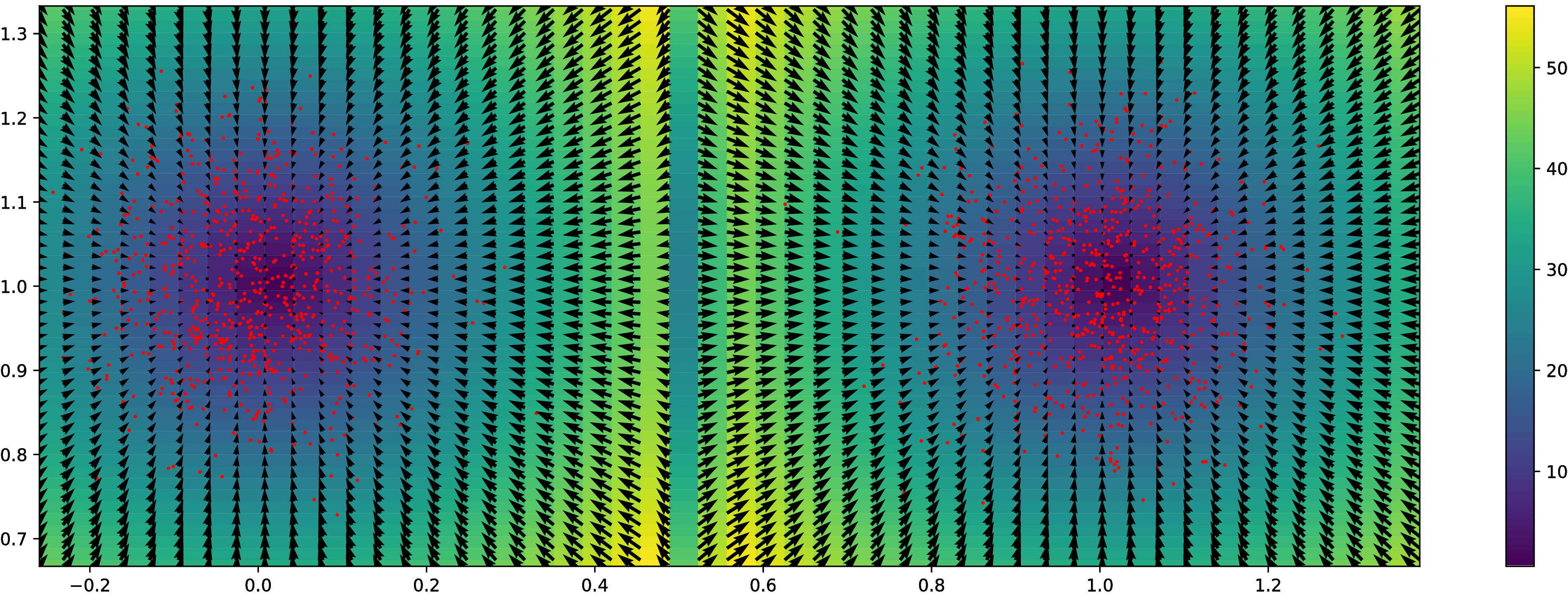
Synthetic experiment: Grid
Normal distributions at vertices of a hypercube in
Synthetic experiment: Grid
Normal distributions at vertices of a hypercube in
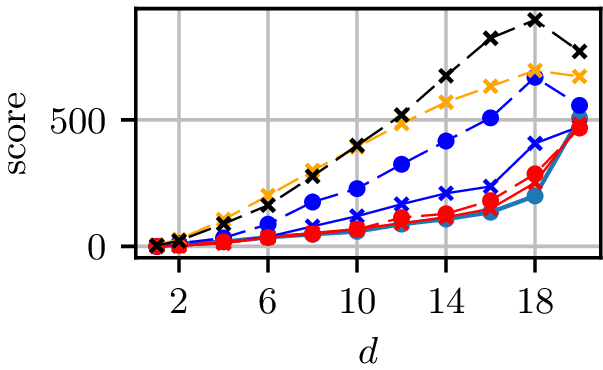
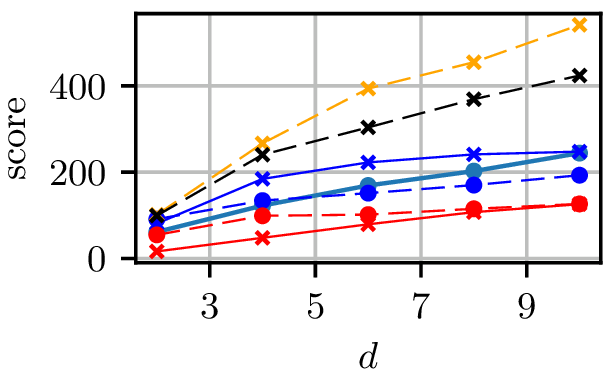
Grid results
Normal distributions at vertices of a hypercube in
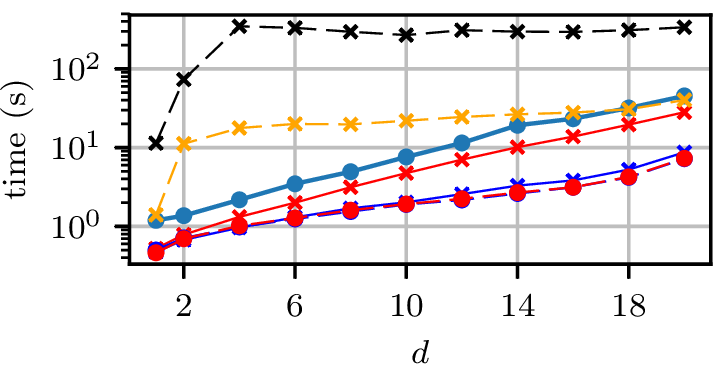
Grid runtimes
Normal distributions at vertices of a hypercube in
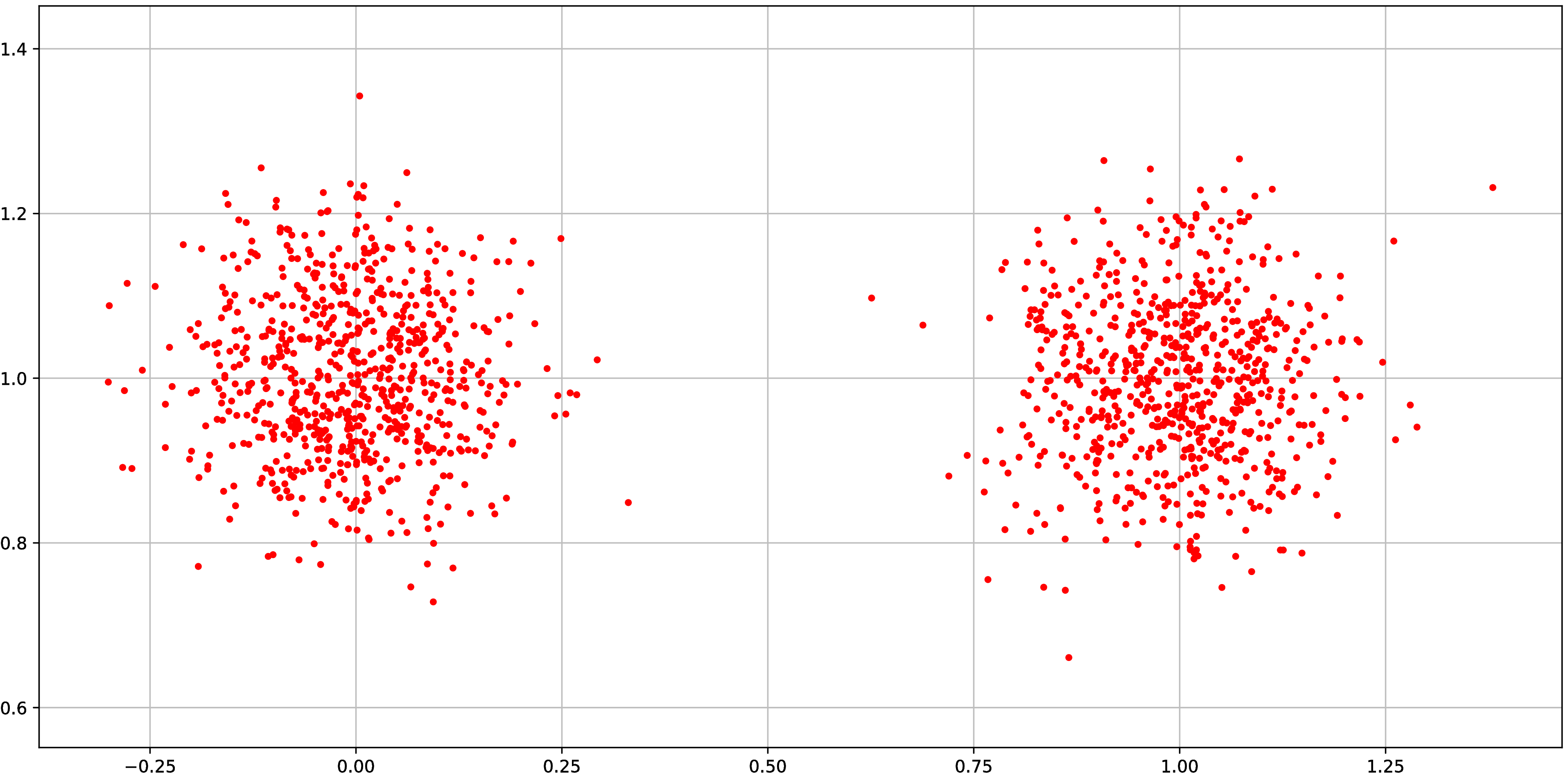
Synthetic experiment: Rings
- Three circles, plus small Gaussian noise in radial direction
- Other dimensions are uniform Gaussian noise
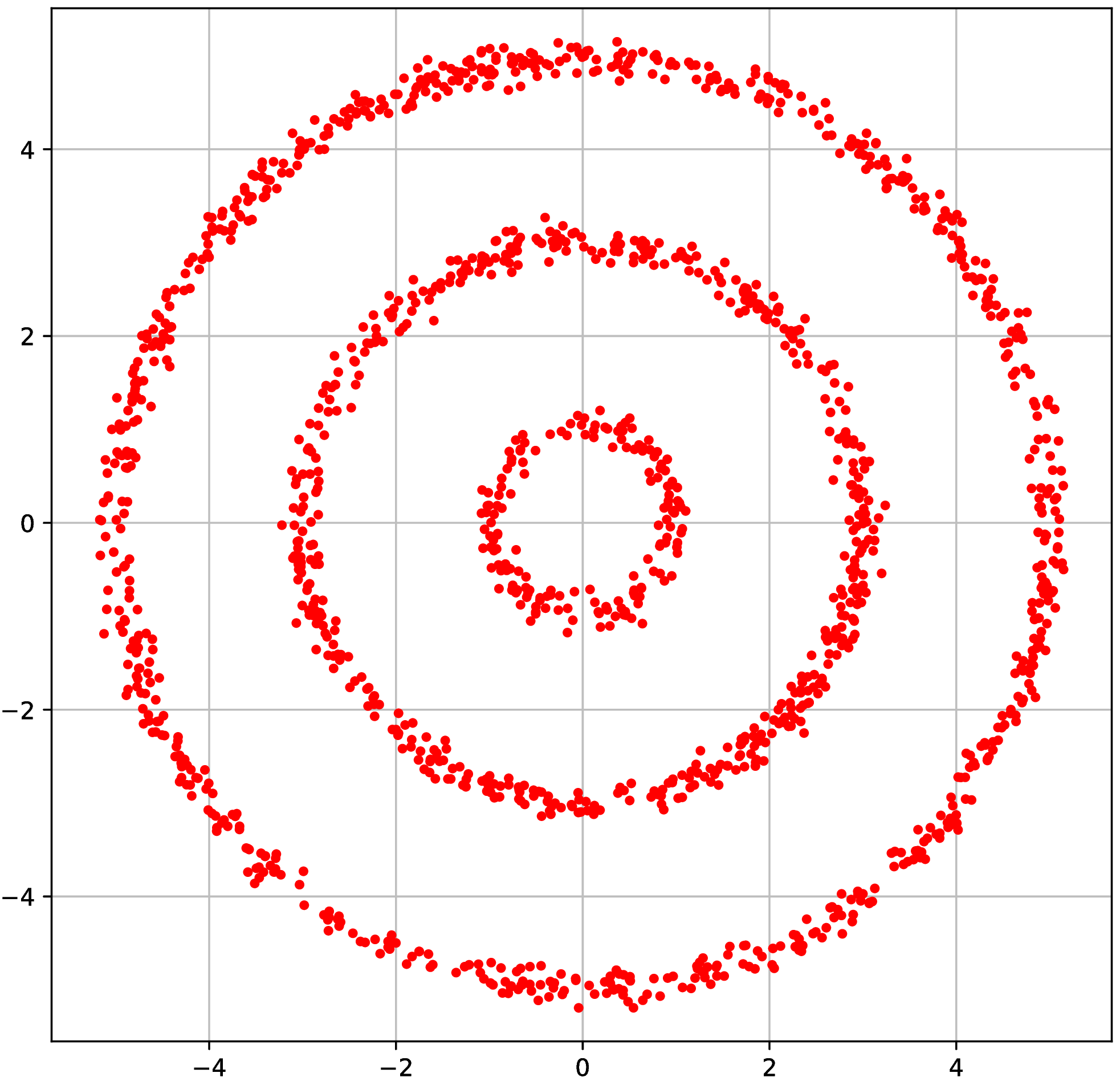
Synthetic experiment: Rings
- Three circles, plus small Gaussian noise in radial direction
- Other dimensions are uniform Gaussian noise
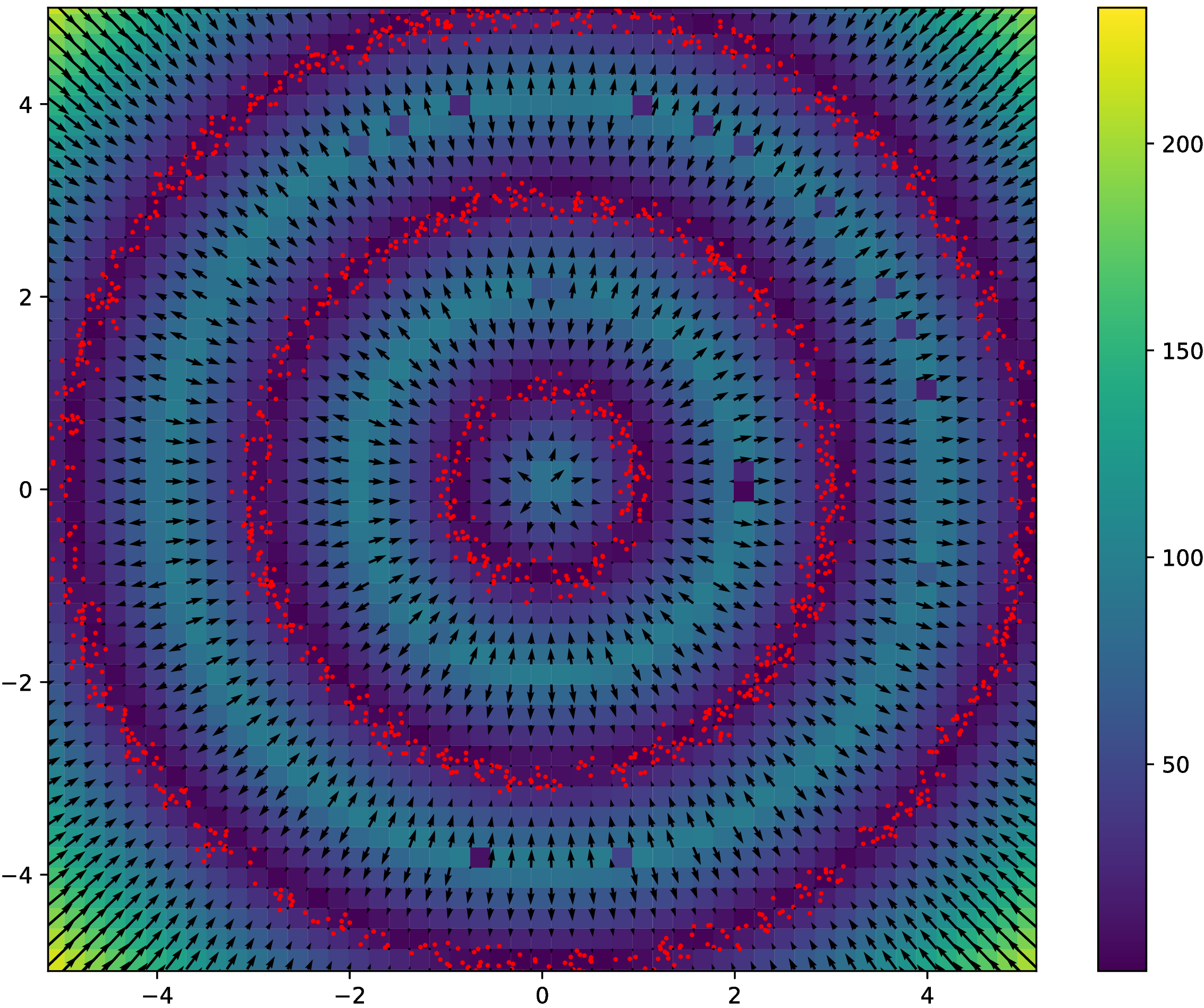
Rings results
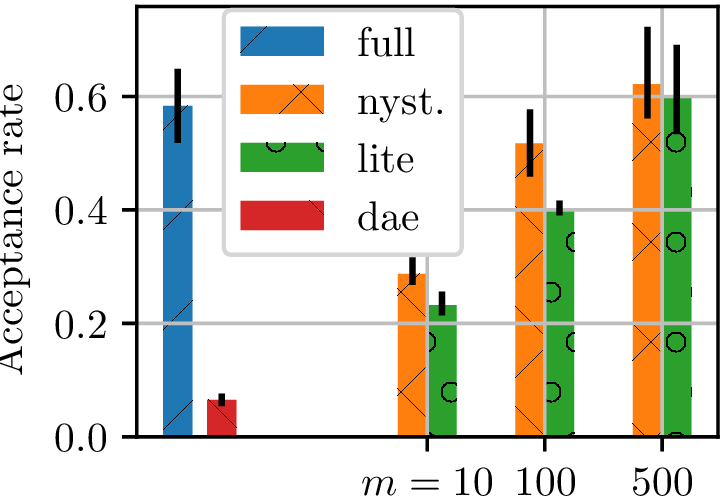
Gradient-free HMC
- Hyperparameter selection for GP classifier on UCI Glass dataset
- Can estimate likelihood of hyperparameters with EP
- Can't get gradients this way
- Fit models to 2000 samples from 40 very-thinned random walks
- Track HMC Metropolis acceptance rate for many trajectories
- higher acceptance rate better model
Gradient-free HMC
Hyperparameter surface
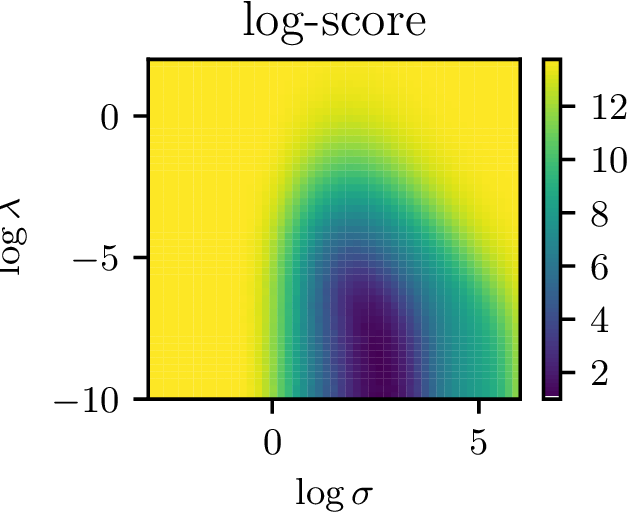
- Nice surface to optimize with gradient descent
- Potentially allows for complex (deep?) kernels
Recap
- Kernel exponential families are rich density models
- Hard to normalize, so maximum likelihood impossible
- Can do score matching, but it's slow
- Nyström gives speedups with guarantees on performance
- Lite version even faster, but no guarantees (yet)
- Could apply to kernel conditional exponential family
Efficient and principled score estimation with kernel exponential families
Dougal J. Sutherland*, Heiko Strathmann*, Michael Arbel, Arthur Gretton
arXiv:1705.08360