Efficient and principled score estimation
with kernel exponential families
Dougal Sutherland
Gatsby unit, UCL
Based on:
- Sutherland*, Strathmann*, Arbel, and Gretton (arXiv:1705.08360)
- Arbel and Gretton (arXiv:1711.05363)
Approximating high dimensional functions, 19 December 2017
Our goal
- A multivariate density model that:
- Is flexible enough to model complex data (nonparametric)
- Is computationally efficient to estimate and evaluate
- Works in high(ish) dimensions
- Has statistical guarantees
| Parametric model | Nonparametric model |
|---|---|
| Multivariate Gaussian | Gaussian process |
| Finite mixture model | Dirichlet process mixture model |
| Exponential family | ??? |
Exponential families
- Can write many densities on as:
- Gaussian:
- Gamma:
- Density only sees data through (and )
- Can we make richer?
Infinitely many features with kernels!
- Kernel: “similarity” function
- e.g. exponentiated quadratic
- For any positive definite on , there's a reproducing kernel Hilbert space of functions on with
- is the infinite-dimensional feature map of

Functions in the RKHS
- Functions in are (closure of) linear combinations of :


Reproducing property
- Functions in are (closure of) linear combinations of :
- Reproducing property:
Kernel exponential families
- Lift parameters from to the RKHS , with kernel :
- Use and , so:
- Covers standard exponential families:
- e.g. normal distribution has
Rich class of densities
- For integrally strictly positive definite that decay to 0,
is dense in the set of distributions that decay like- Examples of :
![]()
- Examples of :

Density estimation
- Given sample , want so that
- Default approach: maximum likelihood
- , are hard to compute
- Ill-posed for characteristic kernels
- Need a way to fit an unnormalized probabilistic model
- Could then estimate once after fitting
Unnormalized density / score estimation
- Don't necessarily need to compute afterwards
- (“energy”) lets us:
- Find modes (global or local)
- Sample (with MCMC)
- …
- The score, , lets us:
- Run HMC when we can't evaluate gradients
- Construct Monte Carlo control functionals
- …
- But again, need a way to find
Score matching in KEFs
- Idea: minimize Fisher divergence
- Under mild assumptions, integration by parts gives
- Estimate with
[Sriperumbudur, Fukumizu, Gretton, Hyvärinen, and Kumar, JMLR 2017]
Score matching in KEFs
- Minimize regularized loss function:
- Thanks to representer theorem, we know


Score matching fit
- Can get an analytic solution to weights in that span:
- has simple closed form
- Solving an linear system takes time!
The Nyström approximation
- Representer theorem: know the best is in
- Nyström approximation: find best in subspace
- If has size- basis, can find coefficients in time
- Worst case: , no improvement
- If ,
- If ,
Nyström basis choice
- Representer theorem: know the best is in
- Reasonable : pick at random, then
- “lite”: pick at random, then


Analysis: Main result
- Well-specified case: there is some so that
- Some technical assumptions on kernel, density smoothness
- is a parameter depending on problem smoothness:
- in the worst case, in the best
- is a parameter depending on problem smoothness:
- Choose basis of size uniformly, :
- Fisher distance :
- Consistent; same rate as full solution
- , KL, Hellinger, ():
- Same rate, consistency for hard problems
- Rate saturates slightly sooner for easy problems
- Fisher distance :
Proof ideas
- Error can be bounded relative to
- Define best estimator in basis :
- New Bernstein inequality for sums of correlated operators
- Approximation key part: covers “most of”
Other main score estimator
- Train a denoising autoencoder with normal noise
- Normalized reconstruction error estimates the score:
- …as long as autoencoder has infinite capacity
- …and is at global optimum
- is like a bandwidth, have to tune it
Experiments
- Two categories:
- Synthetic experiments
- We know true score, and so can compute
- Gradient-free HMC
- We can evaluate quality of proposed gradient steps
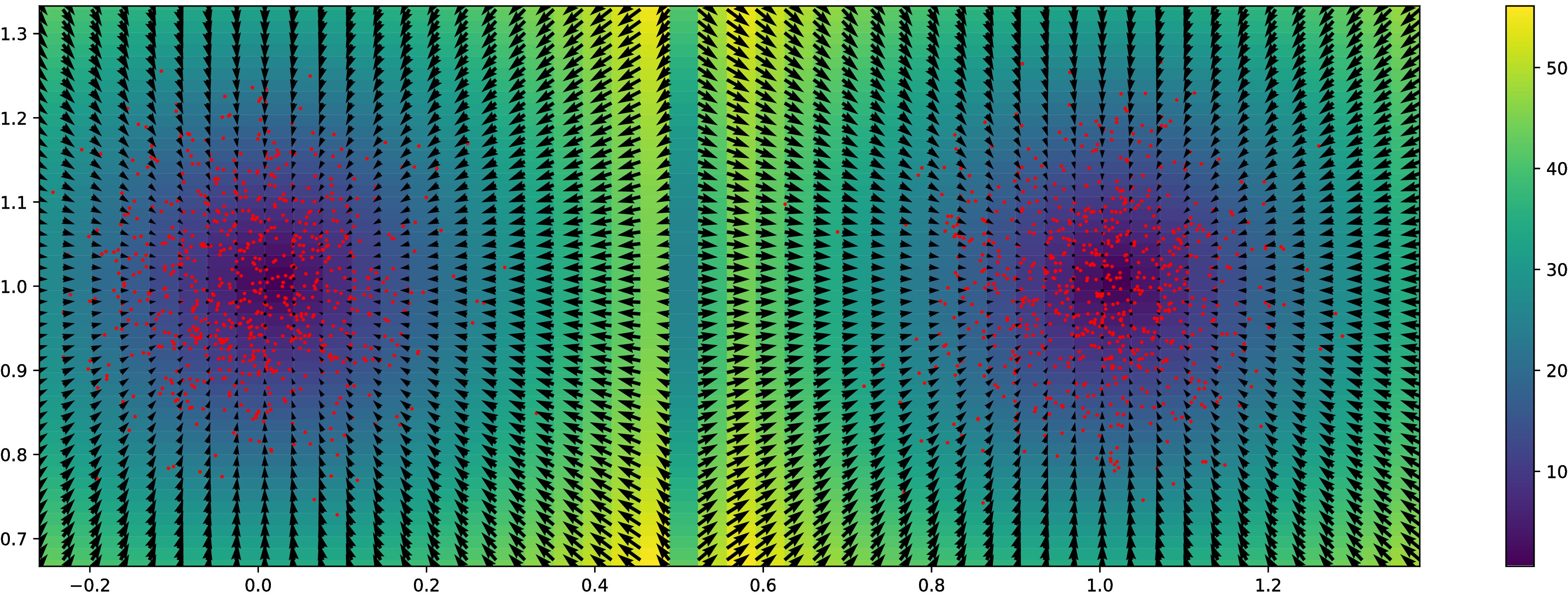
Synthetic experiment: Grid
Normal distributions at vertices of a hypercube in
Synthetic experiment: Grid
Normal distributions at vertices of a hypercube in
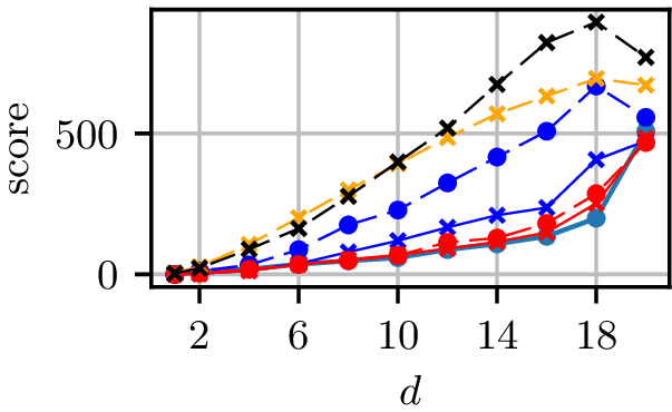
Grid results
Normal distributions at vertices of a hypercube in
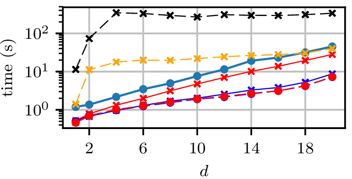
Grid runtimes
Normal distributions at vertices of a hypercube in
Synthetic experiment: Rings
- Three circles, plus small Gaussian noise in radial direction
- Other dimensions are uniform Gaussian noise
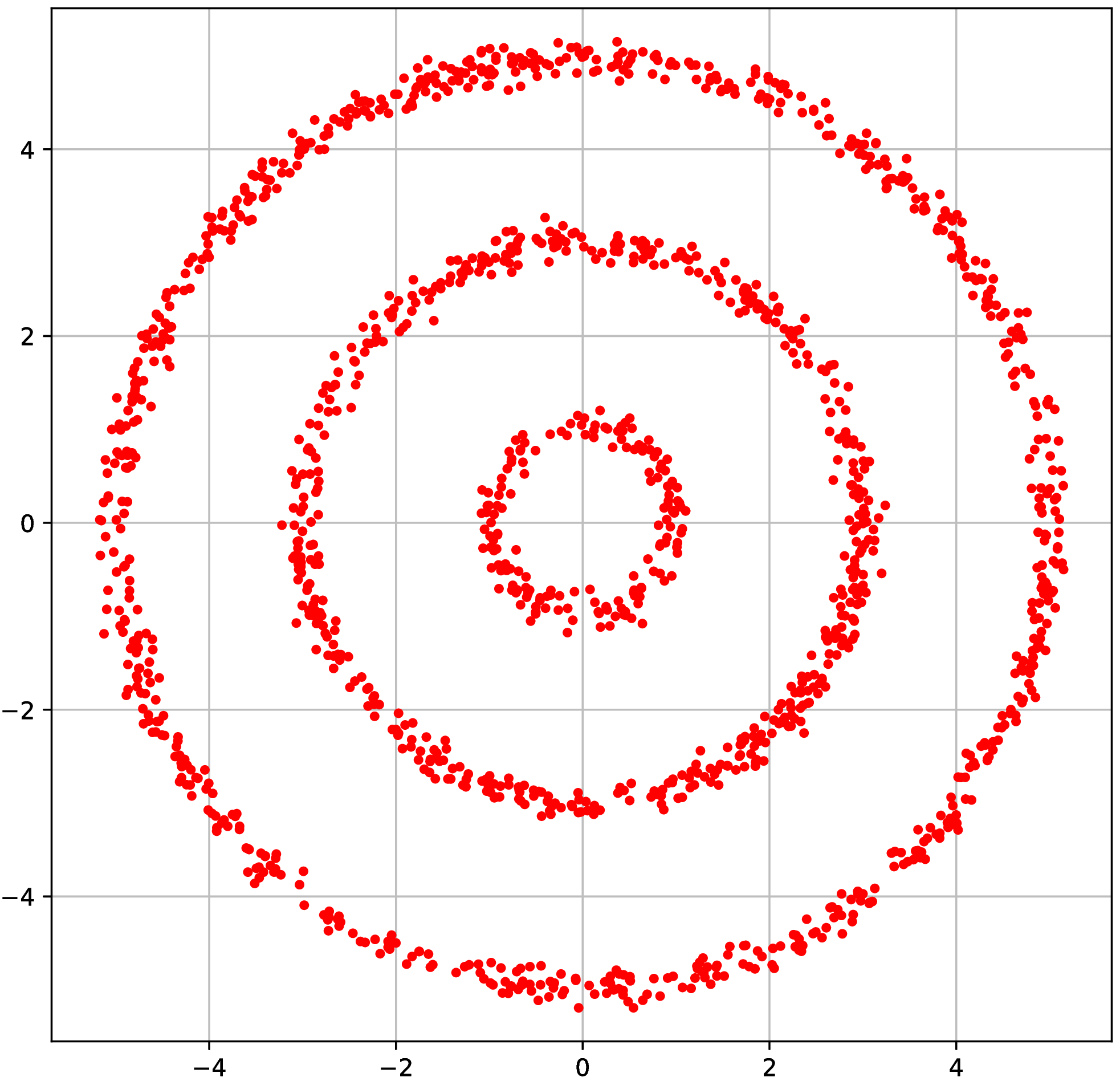
Synthetic experiment: Rings
- Three circles, plus small Gaussian noise in radial direction
- Other dimensions are uniform Gaussian noise
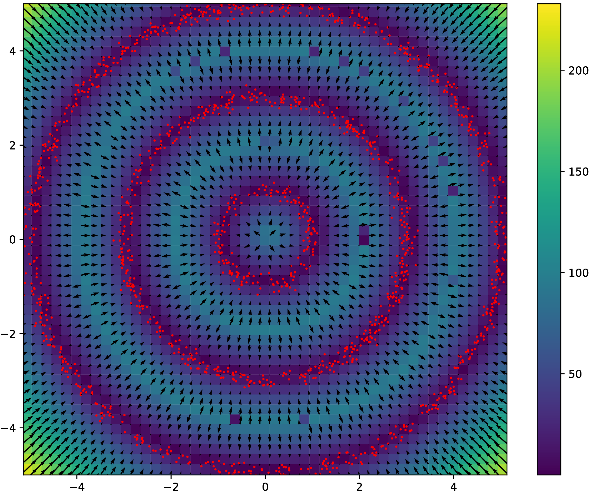
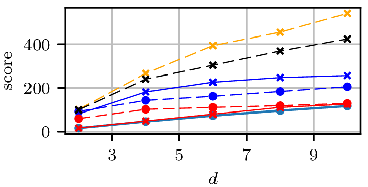
Rings results
Gradient-free HMC
- Want to marginalize out hyperparameter choice for a GP classifier
- Can estimate likelihood of hyperparameters with EP
- Can't get gradients this way: no HMC
- Approximate HMC method [Strathmann et al. NIPS-15]:
- Fit model to estimate scores based on current samples
- Propose HMC trajectories based on score estimate
- Metropolis rejection step accounts for errors in score estimate
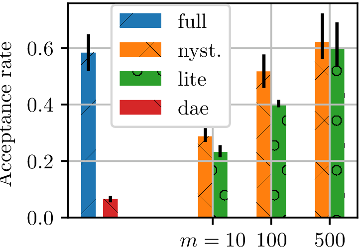
- Our experiment (UCI Glass dataset):
- Fit model on "ground truth" samples
- 2000 samples from 40 very-thinned random walks
- Track HMC acceptance rate for many trajectories
- higher acceptance rate better model
- Fit model on "ground truth" samples
Gradient-free HMC
Hyperparameter surface
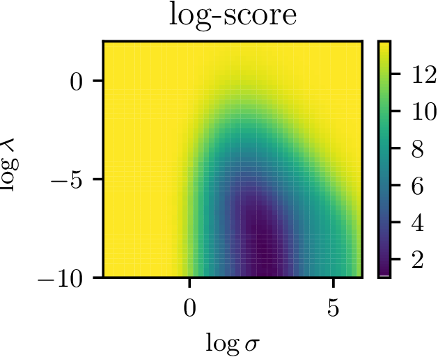
- Nice surface to optimize with gradient descent
- Potentially allows for complex (deep?) kernels
Recap so far
- Kernel exponential families are rich density models
- Hard to normalize, so maximum likelihood intractible
- Can do score matching, but it's slow
- Nyström gives speedups with guarantees on performance
- Lite version even faster, but no guarantees (yet)
Efficient and principled score estimation with kernel exponential families
Dougal J. Sutherland*, Heiko Strathmann*, Michael Arbel, Arthur Gretton
arXiv:1705.08360
Kernel Conditional Exponential Family (arXiv:1711.05363)
Michael Arbel and Arthur Gretton
- often has a graphical structure:
- Estimate each factor independently
Kernel conditional exponential family
- General definition: use joint feature map :
- Proposed particular case:
- Feature map given by:
- is a vector-valued RKHS [Michelli/Pontil 2005]
What loss function to use?
- Obvious approach: minimize
- Problem: expression still depends on
- Instead: minimize
- Zero iff conditional densities are equal for -almost all
- Leads to analytical minimizer of same form as before
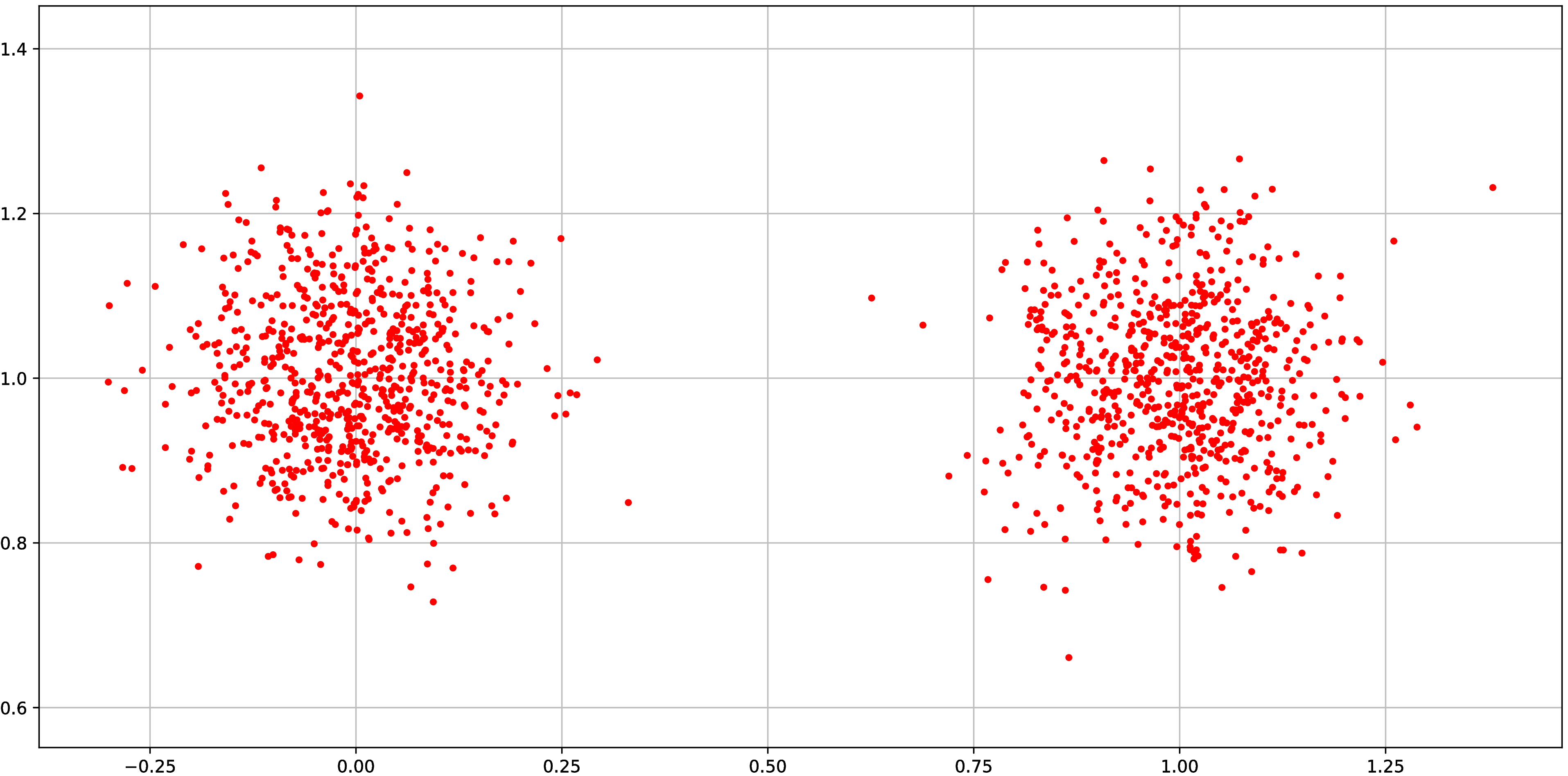
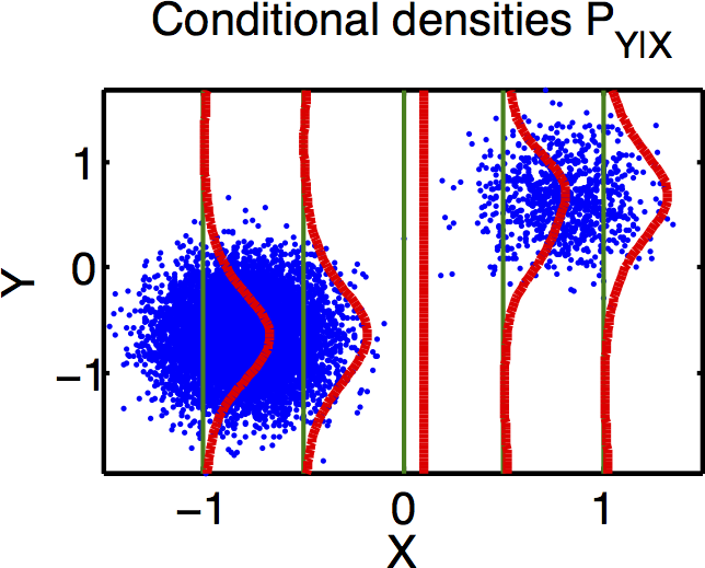
Failure mode of expected conditional score
Failure mode of expected conditional score
Why does it fail?
Loss is
since supports are disjoint, and we drop the normalizer…
Violates assumptions of model, but need to be careful as we approach this situation!
Unconditional vs conditional model
- Parkinsons: biomedical voice measurements from patients with early-stage Parkinson's disease
- Red Wine: physiochemical measurements on wine samples
| Parkinsons | Red Wine | |
|---|---|---|
| Dimension | 15 | 11 |
| Samples | 5,875 | 1,599 |
Unconditional vs conditional model
- Parkinsons:
- Red Wine:
Compare to:
- LSCADE: density ratio estimation, has guarantees [Sugiyama+ 2010]
- RNADE: deep learning, no guarantees [Uria+ NIPS-13]
Negative log likelihoods: (smaller is better; 5 splits)
| Parkinsons | Red Wine | |
|---|---|---|
| KCEF | 2.86 ± 0.77 | 11.8 ± 0.93 |
| LSCDE | 15.89 ± 1.48 | 14.43 ± 1.5 |
| NADE | 3.63 ± 0.0 | 9.98 ± 0.0 |
Sampling: Red Wine
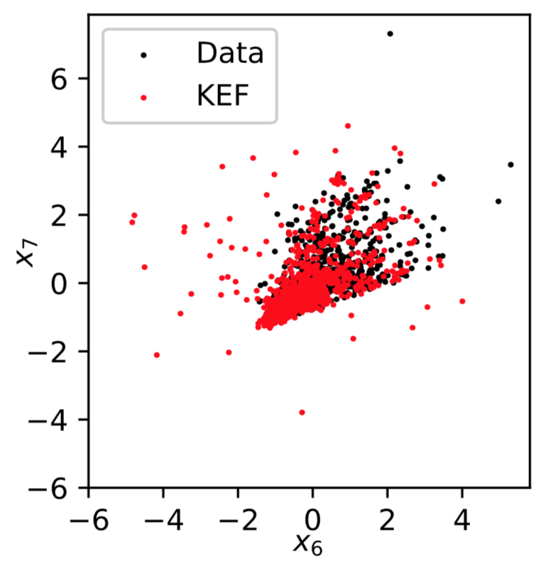
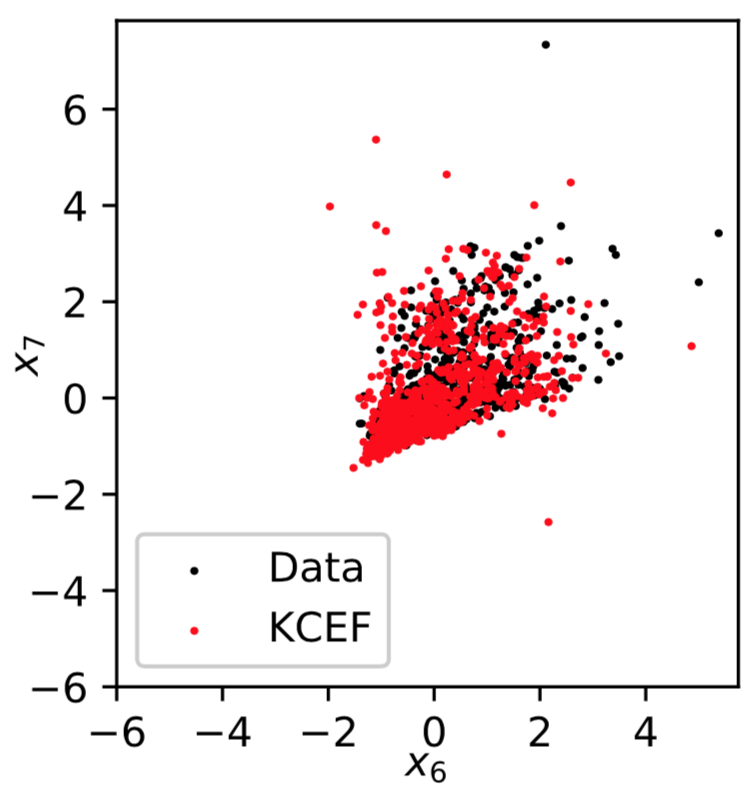
Sampling: Parkinsons
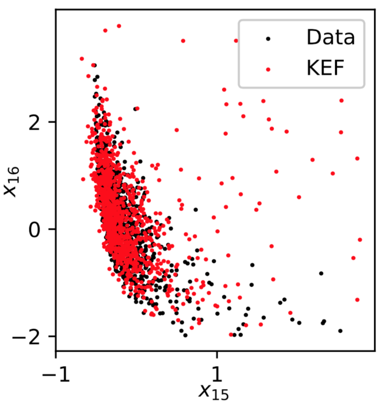
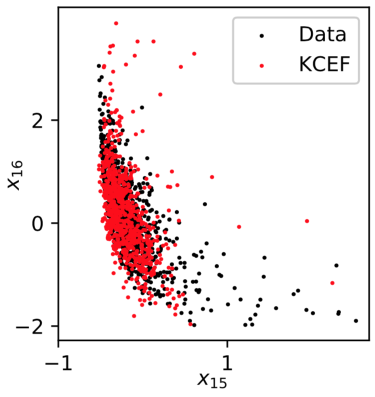
Recap
- Kernel exponential families are rich density models
- Hard to normalize, so need score matching
- Nyström gives speedups with guarantees on performance
- Conditional version: more complex, higher-dimensional models
Efficient and principled score estimation with kernel exponential families
Dougal J. Sutherland*, Heiko Strathmann*, Michael Arbel, Arthur Gretton
arXiv:1705.08360
Kernel Conditional Exponential Family (arXiv:1711.05363)
Michael Arbel and Arthur Gretton