Efficiently estimating densities and scores
with Nyström kernel exponential families
Gatsby unit, University College London

Gatsby Tri-Centre Meeting, June 2018
Our goal
- A multivariate density model that:
- Is flexible enough to model complex data (nonparametric)
- Is computationally efficient to estimate and evaluate
- Works in high(ish) dimensions
- Has statistical guarantees
| Parametric model | Nonparametric model |
|---|---|
| Multivariate Gaussian | Gaussian process |
| Finite mixture model | Dirichlet process mixture model |
| Exponential family | Kernel exponential family |
Exponential families
- Can write many classic densities on as:
- Gaussian:
- Gamma:
- Density only sees data through (and )
- Can we make richer?
Infinitely many features with kernels!
- Kernel: “similarity” function
- e.g. exponentiated quadratic
- Reproducing kernel Hilbert space of functions on with
- is the infinite-dimensional feature map of
- Similarity to all possible inputs :


Kernel exponential families
- Lift parameters from to the RKHS , with kernel :
- Use parameter and sufficient statistic :
- Covers standard exponential families:
- e.g. normal distribution has
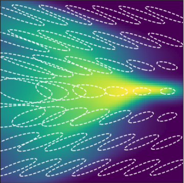
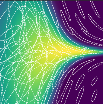
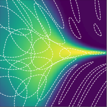
Rich class of densities
- For “strong” that decay to 0,
is dense in the set of continuous densities with tails like
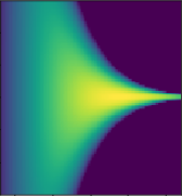
- Examples of with Gaussian :
![]()
- Examples of with Gaussian :

Density estimation
- Given sample , want so that
- Usual approach: maximum likelihood
- , are hard to compute
- Likelihood equations ill-posed for characteristic kernels
- Need a way to fit an unnormalized probabilistic model
- Could then estimate once after fitting
Unnormalized density / score estimation
- Don't necessarily need to compute afterwards
- (“energy”) lets us:
- Find modes (global or local)
- Sample (with MCMC)
- …
- The score, , lets us:
- Run HMC when we can't evaluate gradients
- Construct Monte Carlo control functionals
- …
- But again, need a way to find
Score matching in KEFs
- Idea: minimize Fisher divergence
- Under mild assumptions, integration by parts gives
- Can estimate with Monte Carlo
[Sriperumbudur, Fukumizu, Gretton, Hyvärinen, and Kumar, JMLR 2017]
Score matching in KEFs
- Minimize regularized loss function:
- Representer theorem tells us minimizer of over is


Best score matching fit in subspace
- Best is in
- Can find best
in subspace of dim
in time
- : , time!
Nyström approximation
- Nyström approximation: find fit in different (smaller)
- One choice: pick , at random, then
- “lite”: pick at random, then


Analysis: Main result
- Well-specified case: there is some so that
- Some technical assumptions on kernel, density smoothness
- is a parameter depending on problem smoothness:
- in the worst case, in the best
- is a parameter depending on problem smoothness:
- Choose basis, size uniformly, :
- Fit takes time instead of
- Fisher distance :
- Consistent; same rate as full solution of [Sriperumbudur+ 2017]
- , KL, Hellinger, ():
- Same rate, consistency for hard problems
- Rate saturates slightly sooner for easy problems
Proof ideas
- Error can be bounded relative to
- Define best estimator in basis :
- New Bernstein inequality for sums of correlated operators
- Approximation key part: covers “most of”
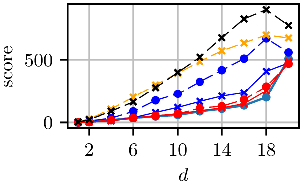
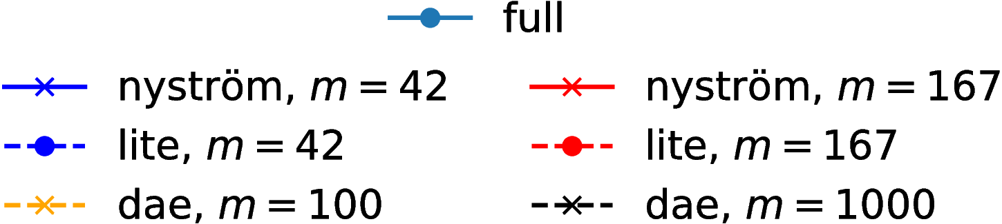
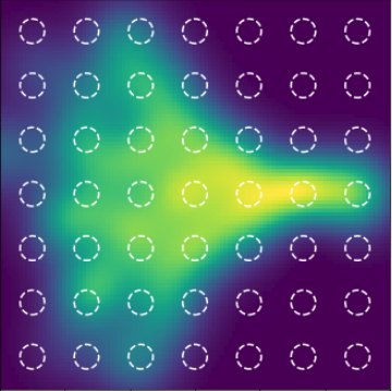
Synthetic experiment: Grid
Normal distributions at vertices of a hypercube in

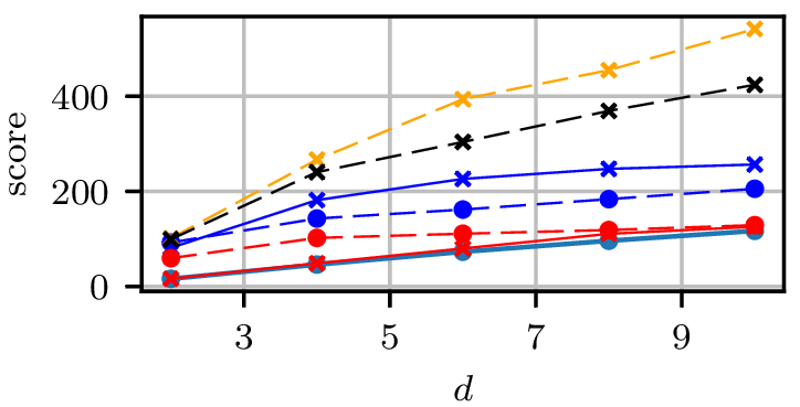
Grid results
Normal distributions at vertices of a hypercube in
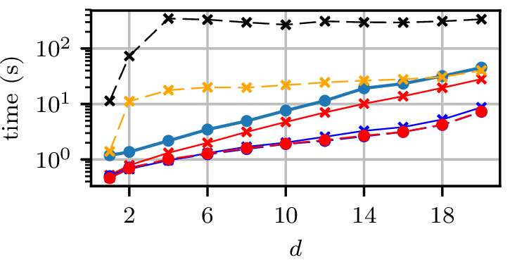
Grid runtimes
Normal distributions at vertices of a hypercube in
Synthetic experiment: Rings
- Three circles, plus small Gaussian noise in radial direction
- Other dimensions are uniform Gaussian noise
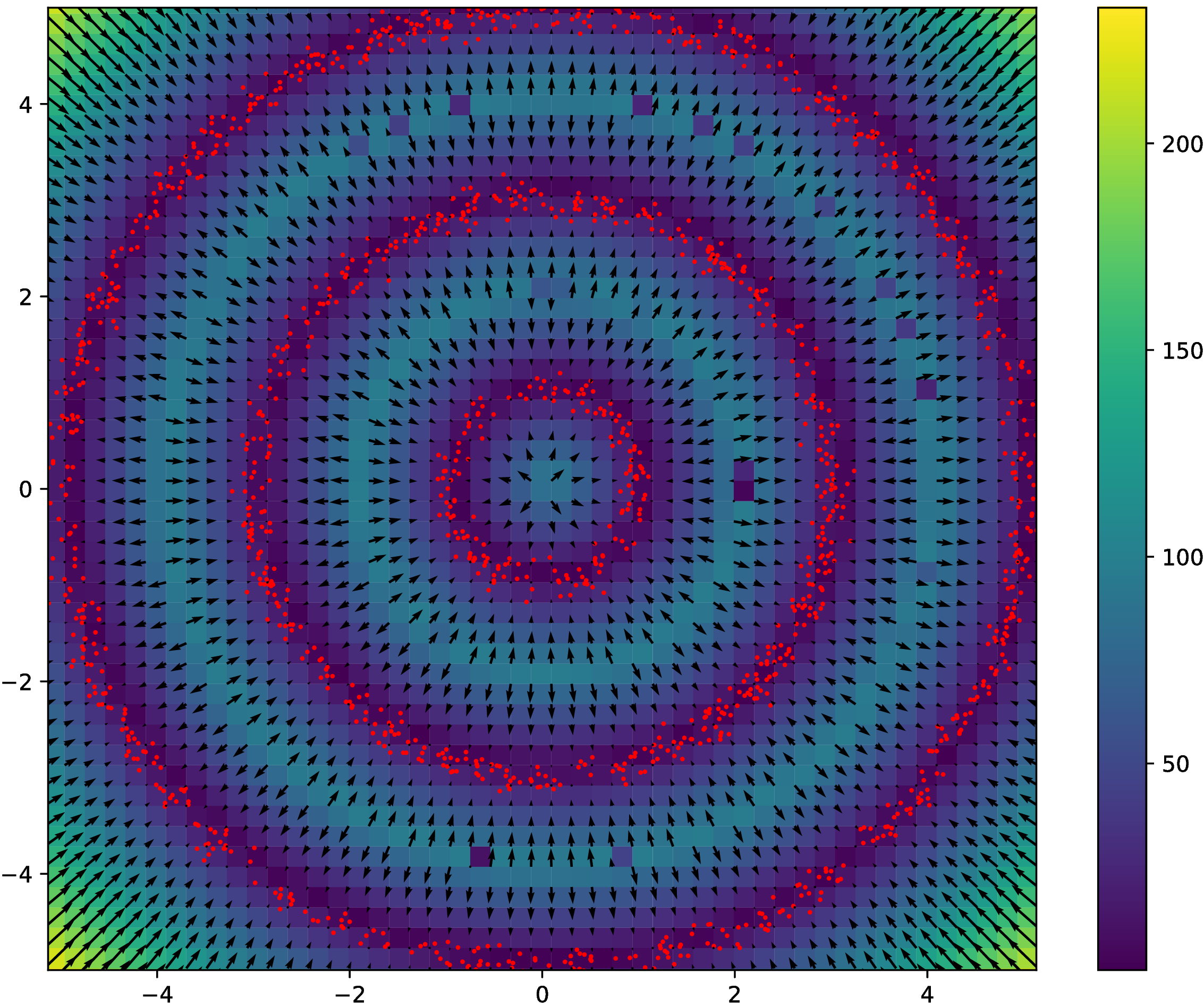
Rings results
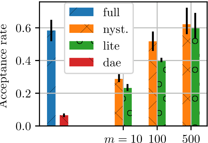
Gradient-free Hamiltonian Monte Carlo
- Want to marginalize out hyperparameter choice for a GP classifier
- Can estimate likelihood of hyperparameters with EP
- Can't get gradients this way: no HMC
- Kernel Adaptive HMC [Strathmann et al. NIPS-15]:
- Fit model to estimate scores based on current samples
- Propose HMC trajectories based on score estimate
- Metropolis rejection step accounts for errors in score estimate
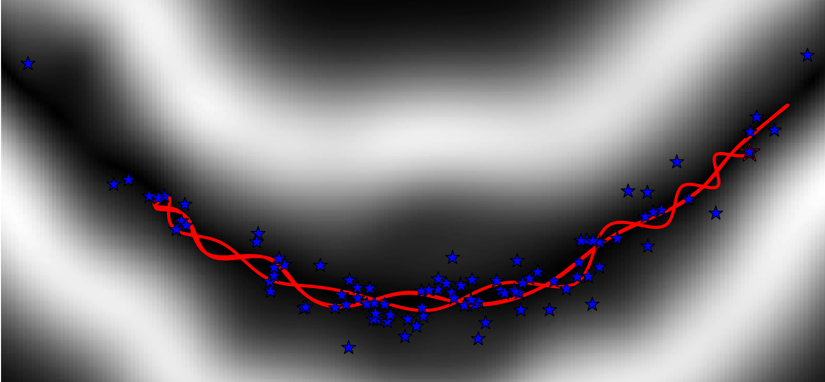
Gradient-free HMC
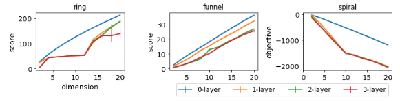
Learning the kernel
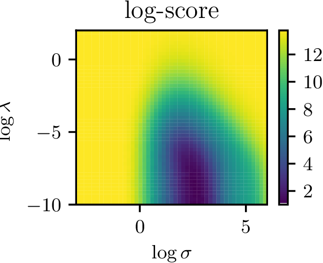
- Nice surface to optimize with gradient descent
Learning deep kernels
Use kernel , with a deep network
Truth
0 layers
1 layer
2 layers
3 layers
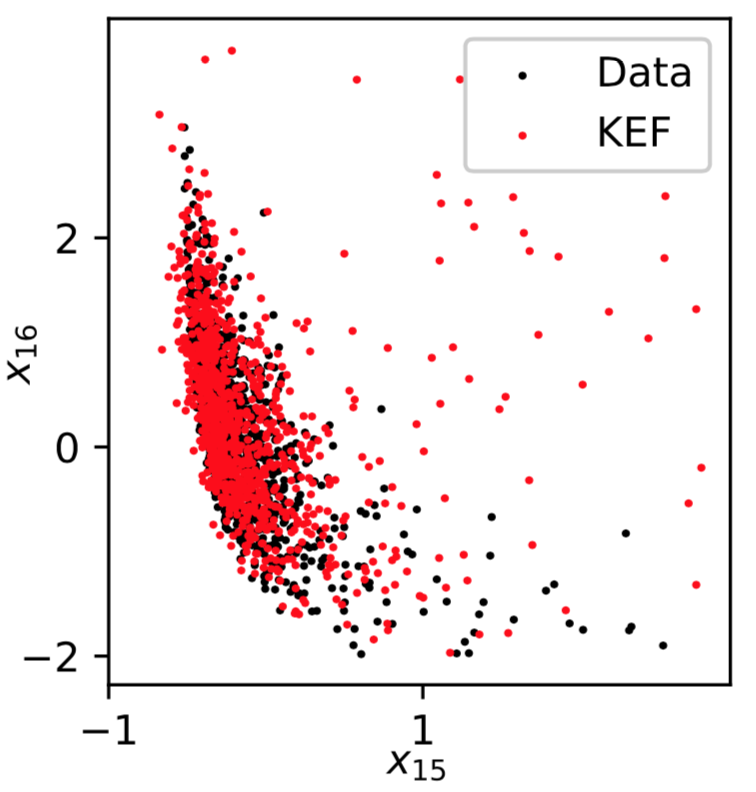
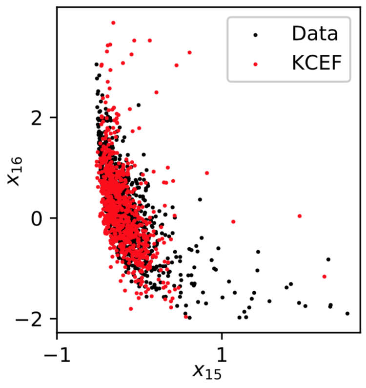
Kernel Conditional Exponential Family
Michael Arbel, Arthur Gretton; AISTATS 2018, arXiv:1711.05363- Add kernel for conditioning variable too
Recap
- Kernel exponential families are rich density models
- Hard to normalize, so maximum likelihood intractible
- Score matching works, but it's slow
- Nyström gives speedups with guarantees on performance
- Lite variant even faster, but no guarantees (yet)
- More complex densities: learn kernel and/or conditional structure
Efficient and principled score estimation
with Nyström kernel exponential families
Dougal J. Sutherland*, Heiko Strathmann*, Michael Arbel, Arthur Gretton
AISTATS 2018; arXiv:1705.08360