Kernel Distances
for Better Deep Generative Models
Based on
“Demystifying MMD GANs”
[ICLR-18]
and
“On gradient regularizers for MMD GANs”
[NIPS-18],
with:
GPSS 2018 - Advances in Kernel Methods, 6 Sep 2018
(Swipe or arrow keys to move in slides; for a menu to jump; to show more.)
Implicit generative models
Given samples from a distribution over ,
want a model that can produce new samples from

Don't necessarily care about likelihoods, interpretability, …
Model: Generator network
Deep network (params ) mapping from noise to images

DCGAN generator [Radford+ ICLR-16]
is e.g. uniform on
Choose by minimizing…something
Loss function
- Can't evaluate likelihood of samples under model
- Likelihood maybe not the best choice anyway [Theis+ ICLR-16]
- Doesn't hurt likelihoods much to take 99% white noise
- Instead, we'll minimize some
 Max-likelihood objective vs WGAN objective [Danihelka+ 2017]
Maximum Mean Discrepancy [Gretton+ 2012]
( is RKHS with kernel )


Can do optimization in closed form:
Deriving MMD
Unbiased estimator of
 |  |  |  |  |  | |
|---|---|---|---|---|---|---|
| 0.6 | 0.5 | 0.2 | 0.4 | 0.2 | |
| 0.6 | 0.7 | 0.4 | 0.1 | 0.1 | |
| 0.5 | 0.7 | 0.3 | 0.1 | 0.2 | |
| 0.2 | 0.4 | 0.3 | 0.7 | 0.8 | |
| 0.4 | 0.1 | 0.1 | 0.7 | 0.6 | |
| 0.2 | 0.1 | 0.2 | 0.8 | 0.6 |
MMD as loss [Li+ ICML-15, Dziugaite+ UAI-15]
Estimate generator based on SGD
with minibatches
, ,
loss
Hard to pick a good kernel for images
MMD GANs: Deep kernels [Li+ NIPS-17]
- Use a class of deep kernels:
- Choose most-discriminative out of those kernels:
- Initialize random generator and representation
- Repeat:
SGD step in to minimize
- times:
- Take SGD step in to maximize
- Take SGD step in to minimize
- times:
- Repeat:
SGD step in to minimize
Smoothness of
- Toy problem in , DiracGAN [Mescheder+ ICML-18]:
- Point mass target , model
- Representation ,
- Kernel


Plain doesn't work [Sutherland+ ICLR-17]:

Wasserstein and WGANs

- WGANs [Arjovsky+ ICML-17],
WGAN-GPs [Gulrajani+ NIPS-17]:
- Update a critic neural network
- Enforce Lipschitz constraint on (more shortly)
- Run SGD to minimize estimate of with that critic
- Update a critic neural network
Enforcing Lipschitz constraint
- One strategy: only optimize over that are -Lipschitz
- Hard to closely specify Lipschitz constant of deep nets
- WGAN [Arjovsky+ ICML-17] tried with simple box constraint
- Also original MMD GAN paper [Li+ NIPS-17]
- WGAN-GP [Gulrajani+ NIPS-17]:
penalize non-Lipschitzness
(with drawn in between the and minibatches)
- Looser constraint than Lipschitz
- Tends to work better in practice
MMD-GAN with gradient control
- If we optimize MMD over kernels giving uniformly Lipschitz critics, loss will be continuous, a.e. differentiable
- Original MMD GAN paper [Li+ NIPS-17] used a box constraint
- We [Binkowski+ ICLR-18] used gradient penalty on critic instead
- Better in practice, but doesn't fix the Dirac problem…

WGAN vs MMD GAN
- Consider linear-kernel MMD GAN, :
- WGAN has:
- Linear-kernel MMD GAN-GP and WGAN-GP almost the same
- MMD GAN “offloads” some of the critic's work to closed-form optimization in the RKHS
Built-in gradient constraints
Lipschitz MMD ()

- Lipschitz MMD:
- Approximation, Gradient-Constrained MMD:
- Variance constraint makes it like a Sobolev norm
- Doesn't quite constrain the Lipschitz constant
Lipschitz MMD ()
GC-MMD,

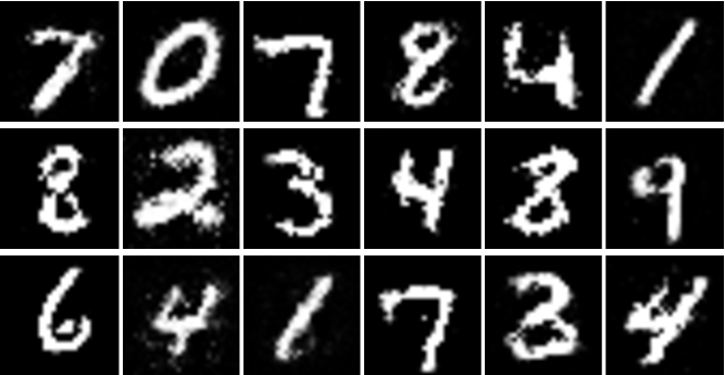
Gradient-Constrained MMD on MNIST
- It's a reasonable distance to optimize:
![]()
- …but this took days to run

Estimating Gradient-Constrained MMD
- Say we have samples
- Let
- Then with has , has , has
- Dropping kernel matrix gives
- Solving this linear system takes time!
Efficent approximation: Scaled MMD
- Using a bit of RKHS theory, can write
- Define scaled MMD as
- Have
Deriving the Scaled MMD:
- Operator given by :
Deriving the Scaled MMD: Lower Bound
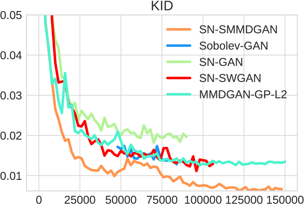
Scaled MMD vs MMD with Gradient Penalty
- When ,


Rank collapse
- Optimization failure we sometimes see on SMMD, GC-MMD:
- Generator doing reasonably well
- Critic filters become low-rank
- Generator corrects it by breaking everything else
- Generator gets stuck


Spectral parameterization [Miyato+ ICLR-18]
- ; learn and freely
- Encourages diversity without limiting representation
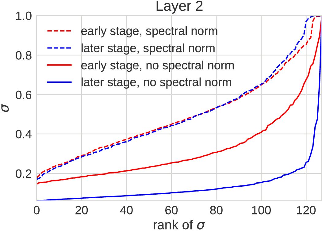
What if we just did spectral normalization?
- , so that ,
- Works well for original GANs [Miyato+ ICLR-18]
- …but doesn't work at all as only constraint in a WGAN
- Limits representation too much
- In the toy problem, constrains to
Implicit generative model evaluation
- No likelihoods, so…how to compare models?
- Main approach:
look at a bunch of pictures and see if they're pretty or not- Easy to find (really) bad samples
- Hard to see if modes are missing / have wrong probabilities
- Hard to compare models beyond certain threshold
- Need better, quantitative methods
Inception score [Salimans+ NIPS-16]
- Previously standard quantitative method
- Based on ImageNet classifier label predictions
- Classifier should be confident on individual images
- Predicted labels should be diverse across sample
- No notion of target distribution
- Scores completely meaningless on LSUN, Celeb-A, SVHN, …
- Not great on CIFAR-10 either
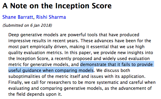
Fréchet Inception Distance (FID) [Heusel+ NIPS-17]
- Fit normals to Inception hidden layer activations of and
- Compute Fréchet (Wasserstein-2) distance between fits
- Meaningful on not-ImageNet datasets
- Estimator extremely biased, tiny variance
- ,


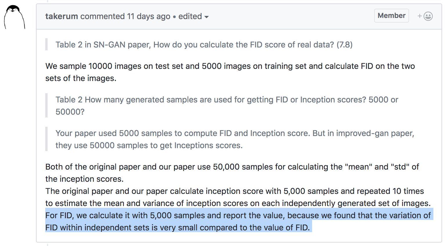
New method: Kernel Inception Distance (KID)
- between Inception hidden layer activations
- Use default polynomial kernel:
- Unbiased estimator, reasonable with few samples
- (Almost) in tensorflow.contrib.gan.eval (tensorflow#21066)

Automatic learning rate adaptation with KID
- Models need appropriate learning rate schedule to work well
- Automate with three-sample MMD test [Bounliphone+ ICLR-16]:

| CIFAR-10 | Small | Big |
|---|---|---|
| WGAN-GP |  .116 ± .002 | 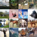 .026 ± .001 |
| MMD GAN-GP | 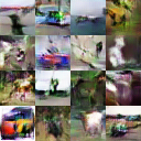 .032 ± .001 | 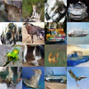 .027 ± .001 |
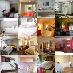
| LSUN Bedrooms | Small | Big |
|---|---|---|
| WGAN-GP |  .370 ± .003 |  .039 ± .002 |
| MMD GAN-GP | 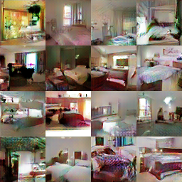 .091 ± .002 | .028 ± .002 |
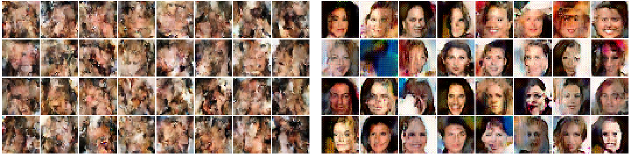
Training on CelebA
CelebA Samples
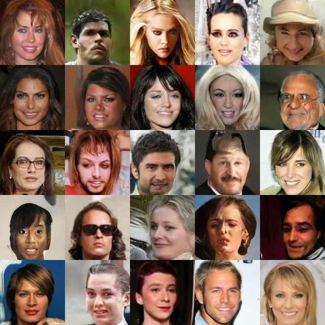
KID: 0.006
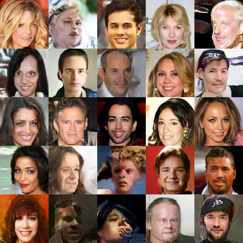
KID: 0.022
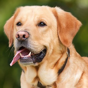
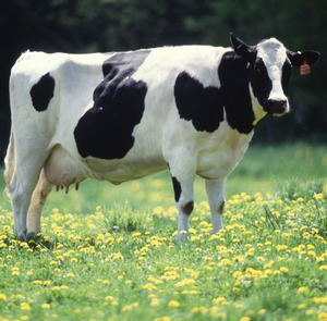
ImageNet Samples
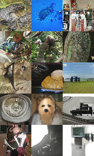
KID: 0.035
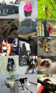
KID: 0.044
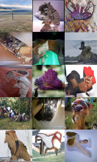
KID: 0.047
Demystifying MMD GANs
[ICLR-18]
Mikołaj Bińkowski*,
Dougal J. Sutherland*,
Michael Arbel,
Arthur Gretton
github.com/mbinkowski/MMD-GAN
- MMD GANs do some optimization in closed form
- Can handle smaller critic networks
- Not in this talk: study of gradient bias for WGAN, MMD GAN
- Unbiased evaluation and learning rate adaptation with KID
On gradient regularizers for MMD GANs
[NIPS-18]
Michael Arbel,
Dougal J. Sutherland,
Mikołaj Bińkowski,
Arthur Gretton
github.com/MichaelArbel/Scaled-MMD-GAN
- Gradient control is important
- Scaled MMD does it in closed form, seems to help a lot
- Spectral normalization plays nice with SMMD
Estimator bias
- Bellemare+ [2017] say that:
- WGANs have biased gradients
- which can lead SGD to wrong minimum even in expectation
- but Cramér GANs have unbiased gradients
- Cramér GAN MMD GAN with particular kernel
- We show:
- Gradients of fixed critic, , are unbiased
- Gradients of optimized critic, , are biased
- Exact same situation for WGAN and MMD GAN
Unbiasedness theorem for fixed critic
- For almost all feedforward architectures ,
- Works for ReLU, max-pooling, …
- For any distributions , with ,
- For most kernels used in practice,
- Includes linear kernel, RBF, RQ, distance kernel, …
- For Lebesgue-almost all parameters :
- , so:
- , unbiased (WGANs)
- unbiased
Proof of unbiasedness theorem
- Can't use standard argument: needs differentiable in a neighborhood of for almost all inputs
- But take
- Fixed : differentiable everywhere but


- might have probability
Proof of unbiasedness theorem
- Instead: Show gradient exchanges when differentiable in for almost all inputs, using Lipschitz properties of the network
- Then show the set of non-differentiable has 0 measure, with a bit of geometry
- Example: for , is a critical point:


Proof of unbiasedness theorem
- By Fubini theorem, only need to show:
- For fixed input , differentiable for almost all
- Recall: , with piecewise smooth :


- case 1: inside domain of analyticity
- case 2: on boundary
- case 3: crosses the boundary:
- in a union of manifolds of 0 measure
Gradient bias for “full” loss
- Recall
- Estimator splits data:
- Pick on train set, estimate on test set
- GAN test set: current minibatch
- Estimator splits data:
- Showed: unbiased for any fixed
- Now: is biased
- Estimators have non-constant bias iff gradients are biased
- Will show is biased
Bias of
- Eval on test set is unbiased:
- But training introduces bias:
- If , estimator must be biased down


- Probably not a big deal in practice
- No (direct) bias due to minibatch size
- Can decrease bias by training critic longer
- But informs theory
- Convergence based on SGD of made difficult
Non-existence of an unbiased IPM estimator
- Beautiful argument of Bickel & Lehman [Ann. Math. Stat 1969]:
- Let ,
- Suppose ; then
- But isn't a polynomial
- So no unbiased can exist – though can