Below we provide source code implementing the extended Projection Pursuit Regression (ePPR) algorithm and simulated data to test its functionality. The simulated data are the natural images and responses with the reference noise level used in Rapela et al. 10. The code runs on R, an environment for statistical computing and graphics. To test ePPR, follow the next steps.

 

1. Download R from http://www.r-project.org/.
1. Click on the "Download, Packages CRAN" link on the left navigator panel.
2. Select the mirror closer to you.
3. Select you operating system (Linux, Mac, Windows),
4. Select the subdirectory "base".
5. Click on the "Download R" link.
2. Install R. The installation is extremely easy, but if necessary check the installation instructions.
3. Download source code for ePPR (save this file in a working directory with the name ePPRFunctions.R).
4. Download the simulated data --images (94 M) plus responses-- and driver script. Save these files in the working directory with the names xNatural.dat, yMFR0.56MIF4.26.dat, and doDemo.R, respectively.
   
5. Run R from the working directory.
   
   • For Windows: right-click the R shortcut on your desktop, select "Properties", and at the end of the Target field (after any final double quote, and separated by a space) insert the text: --sdi --max-mem-size=2Gb. Next, double click on the R shortcut to start R (a Warning could appear indicating that --max-mem-size is too large, but it is not a problem). Finally, in R select the menu "File" and option "Change dir", browse to the working directory, and press the OK button.

   • For Linux: in a terminal cd to the working directory and type R.
   • For Mac: double click on the R icon to start R. Then, from the "Misc" menu select "Change working directory ...", browse to the working directory, and press "Open".
     
6. Finally in the command window of R, type:
source("doDemo.R")

Some remarks:

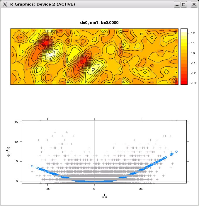
• The driver script will give you the option of plotting the nonlinear functions and filters estimated by the FIT_NEW_TERM procedure (see Appendix B of Rapela et al. 2010) as the algorithm progresses. The figure below shows one of these pairs of nonlinear functions and filters.
  Note: these plots will significantly slow down ePPR. In a personal computer with 3 GB of memory and a 3 GHz processor this estimation takes 45 minutes without plots, and 160 minutes with plots.
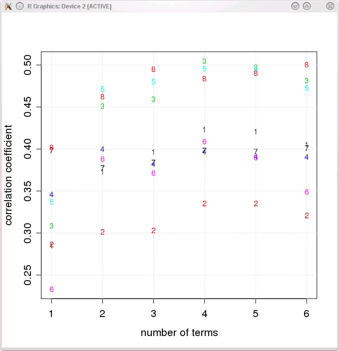
• When the ePPR algorithm finishes, the driver script will plot the correlation coefficients between predictions of the models returned by the BACKWARD_STEPWISE procedure (see Appendix B of Rapela et al. 2010) and cell responses.

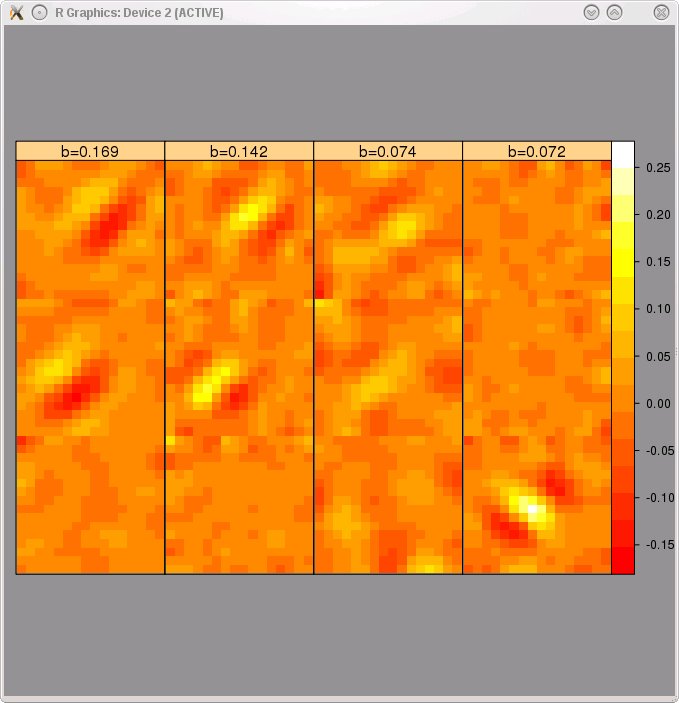
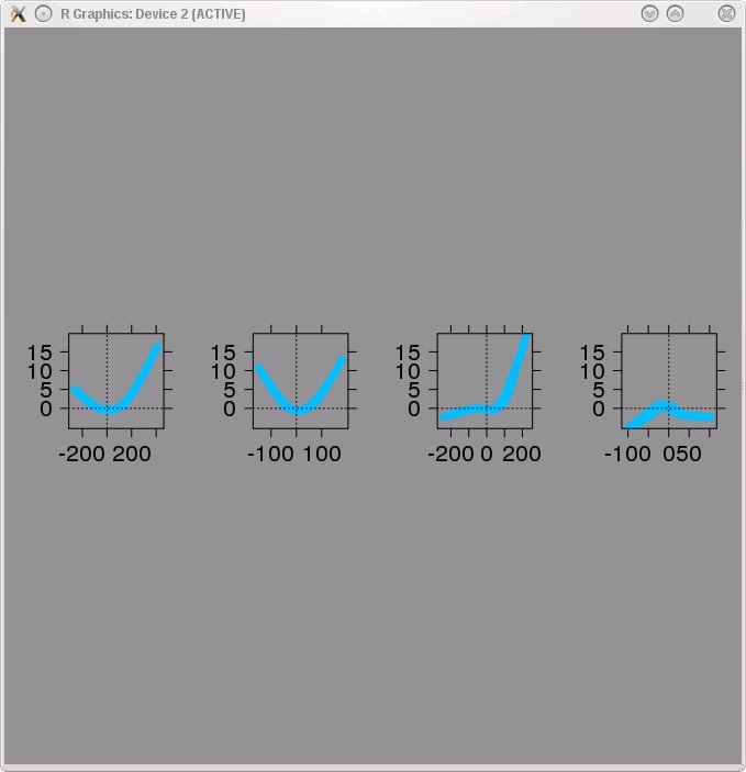
• The driver script will allow you to plot the filters and nonlinear functions of any of the models returned by the BACKWARD_STEPWISE procedure. The filters and nonlinear functions of the model with 4 terms are shown below. This model contains one spurious term (3rd filter and nonlinear function from the left). To remove spurious terms we used the "Removal of spurious terms" procedure described in Section 7.6 of Rapela et al. 2010.

• If you want to use other data, create a first ASCII tab-separated file with one image per row and a second ASCII file with one response per row. Then copy doDemo.R to demoYourCell.R. In demoYourCell.R replace 'xNaturalSequence.dat' by the name of your images file, and replace 'yMFR0.56MIF4.26.dat' by the name of your responses file. Finally, in the R command window type source("doDemoYourCell.R").
  Images do not need to be whitened or weighted according to their corresponding responses, as opposed to spike triggered techniques.
• If you need help processing your data contact Joaquín Rapela.