Generative models
- Start with a bunch of examples:
- Want a model for the data:
- Might want to do different things with the model:
- Find most representative data points / modes
- Find outliers, anomalies, …
- Discover underlying structure of the data
- Impute missing values
- Use as prior (semi-supervised, machine translation, …)
- Produce “more samples”
- …
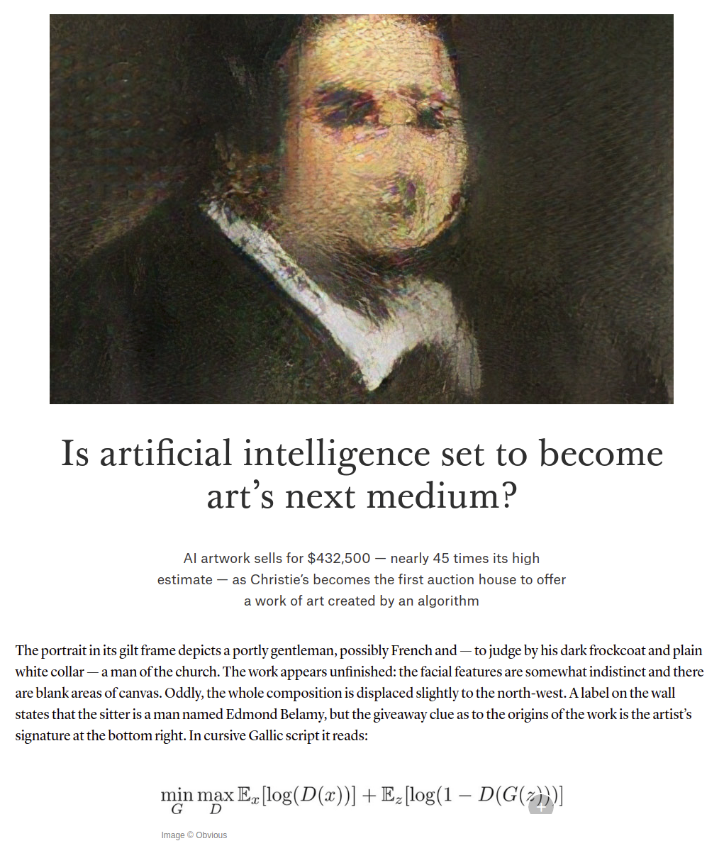
Why produce samples?
![]()
Generative models: a traditional way
- Maximum likelihood:
- Equivalent:
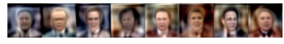
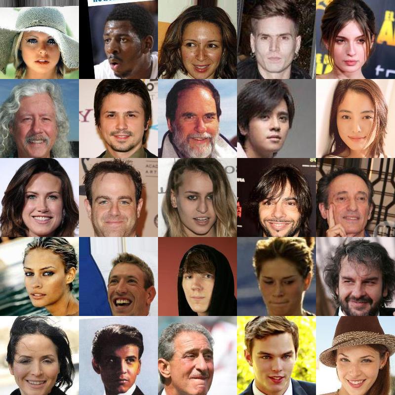
Traditional models for images
- 1987-style generative model of faces (Eigenface via Alex Egg)
![]()
- Can do fancier versions, of course…
- Usually based on Gaussian noise loss
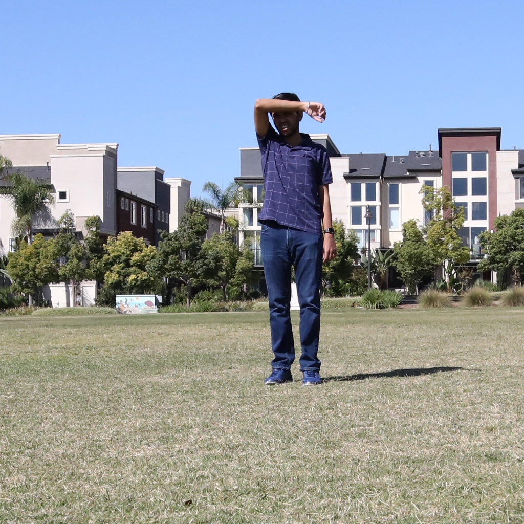
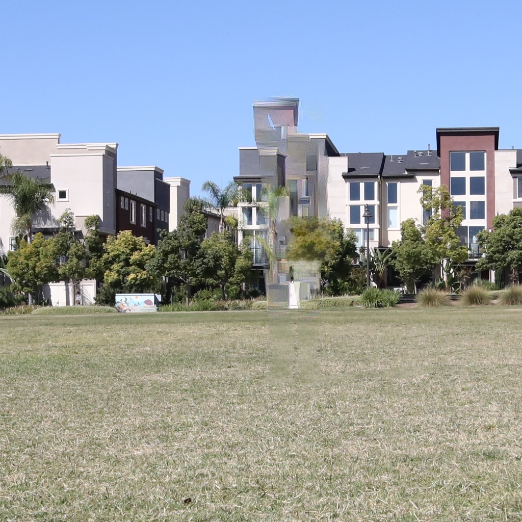
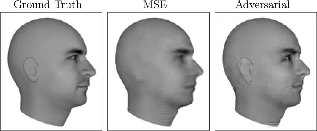
A hard case for traditional approaches
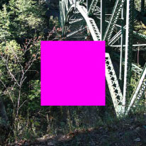
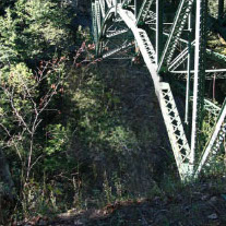
- One use case of generative models is inpainting [Harry Yang]:
- loss / Gaussians will pick the mean of possibilities
Generator ()
![]()
Discriminator
![]()
Target ()
![]()
Is this real?![]()
No way!
:( I'll try harder…
⋮
Is this real?![]()
Umm…
Aside: deep learning in one slide
- MLCC so far: models ,
- is an activation function:
- Classification usually uses log loss (cross-entropy):
- Optimize with gradient descent
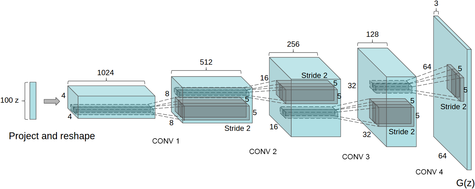
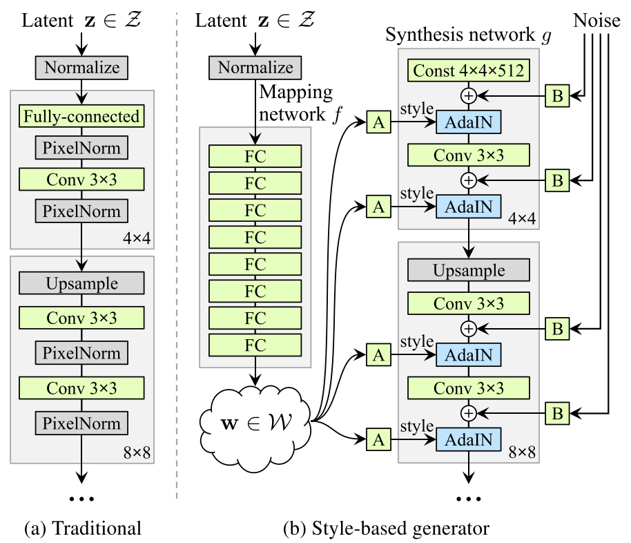
Generator networks
- How to specify ?
![]()
- ,
GANs in equations
- Tricking the discriminator:
- Using the generator network for :
- Can do alternating gradient descent!
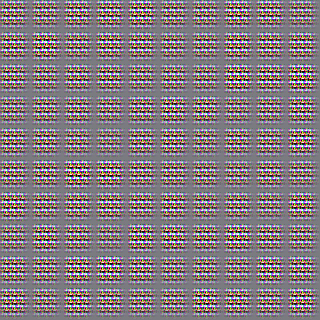
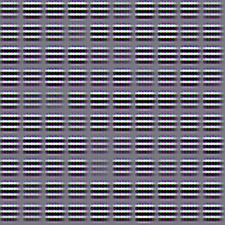
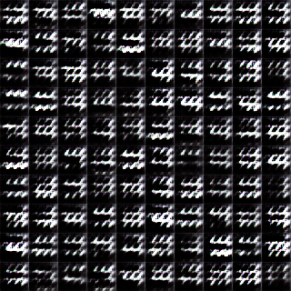
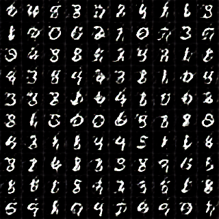
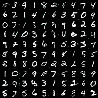
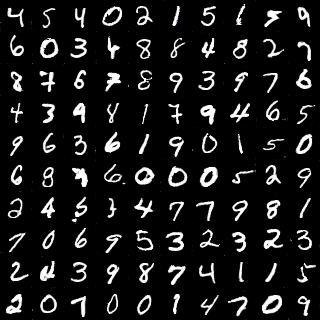
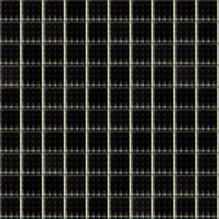
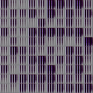
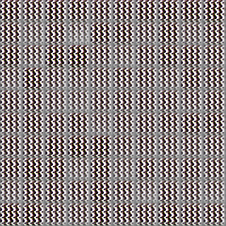
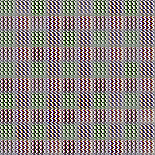
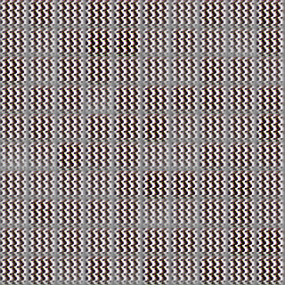
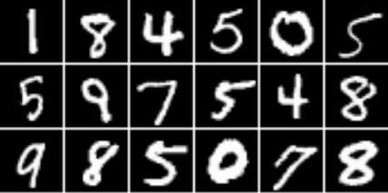
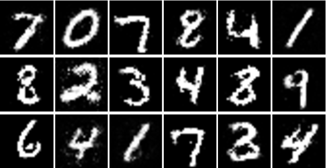
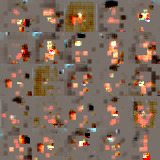
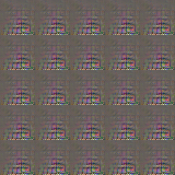
Training instability
Running code from [Salimans+ NeurIPS-16]:
![]()
Run 1, epoch 1
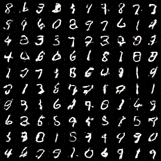
![]()
Run 1, epoch 2
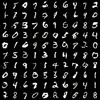
![]()
Run 1, epoch 3
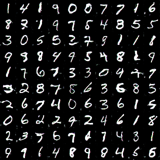
![]()
Run 1, epoch 4
![]()
Run 1, epoch 5
![]()
Run 1, epoch 6
![]()
Run 1, epoch 11
![]()
Run 1, epoch 501
![]()
Run 1, epoch 900
![]()
Run 2, epoch 1
![]()
Run 2, epoch 2
![]()
Run 2, epoch 3
![]()
Run 2, epoch 4
![]()
Run 2, epoch 5
One view: distances between distributions
- What happens when is at its optimum?
- If distributions have densities,
- If stays optimal throughout, tries to minimize
which is
Jensen-Shannon divergence
- If and have (almost) disjoint support
so
Discriminator point of view
Generator ()
![]()
Discriminator
![]()
Target ()
![]()
Is this real?![]()
No way!
:( I don't know how to do any better…
How likely is disjoint support?
- At initialization, pretty reasonable:
:
![]()
:
![]()
- Remember we might have
- For usual , is supported on a countable union of
manifolds with dim - “Natural image manifold” usually considered low-dim
- No chance that they'd align at init, so
A heuristic partial workaround
- Original GANs almost never use the minimax game
- If is near-perfect, near instead of
![]()
- When is near-perfect, makes it unstable instead of stuck
Solution 1: the Wasserstein distance
is a -Lipschitz critic function
Turns out is continuous: if , then
Wasserstein GANs
- Idea: turn discriminator into a critic
- Need to enforce
- Easy ways to do this are way too stringent
- Instead, control on average, near the data
- Specifically: ,
Solution 2: add noise
- Make the problem harder so there's no perfect discriminator
- Use , for some independent, full-dim noise
- But…how much noise to add? Also need more samples.
- If and we take , get
- Same kind of gradient penalty!
- Can also simplify to e.g.
Solution 3: Spectral normalization [Miyato+ ICLR-18]
- Regular deep nets:
- Spectral normalization:
- is the spectral norm
- Guarantees
- Faster to evaluate than gradient penalties
- Not as well understood yet
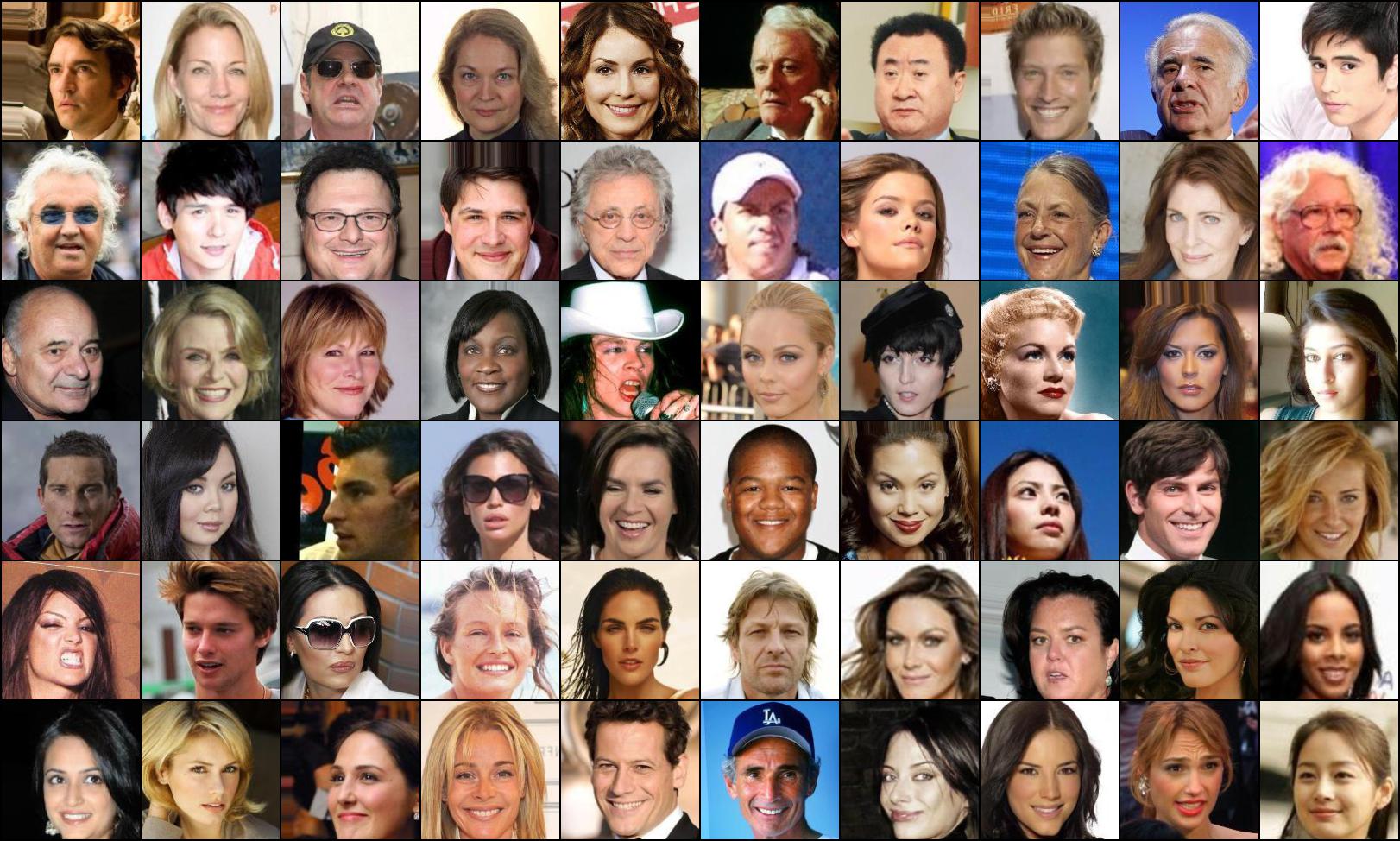
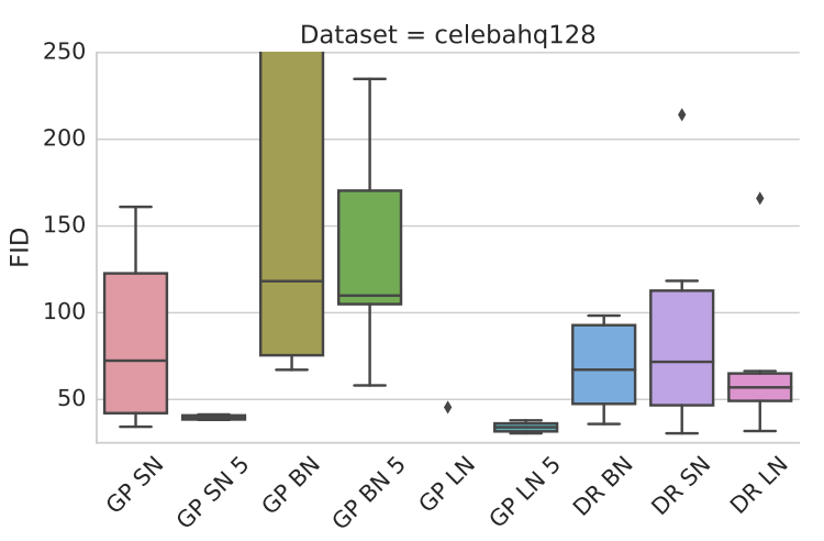
How to evaluate?
![]()
- Consider distance between distributions of image features
- Features from a pretrained ImageNet classifier
- FID:
- Estimator very biased, small variance
- KID: use Maximum Mean Discrepancy instead
- Similar distance with unbiased, ~normal estimator!
![]()
Maximum Mean Discrepancy
is smoothness induced by kernel
Optimal analytically:
Estimating MMD
- No need for a discriminator – just minimize !
- Continuous loss
Generator ()
![]()
Critic
![]()
Target ()
![]()
How are these?![]()
![]()
![]()
Not great!
:( I'll try harder…
⋮
MMD loss with a smarter kernel
- from pretrained Inception net
- simple: exponentiated quadratic or polynomial
![]()
![]()
- Don't just use one kernel, use a class parameterized by :
- New distance based on all these kernels:
- Turns out that isn't continuous:
have but
- Scaled MMD GANs [Arbel+ NeurIPS-18]
correct with a gradient penalty to make it continuous
Why MMD GANs?
- “Easy parts” of the optimization done in closed form
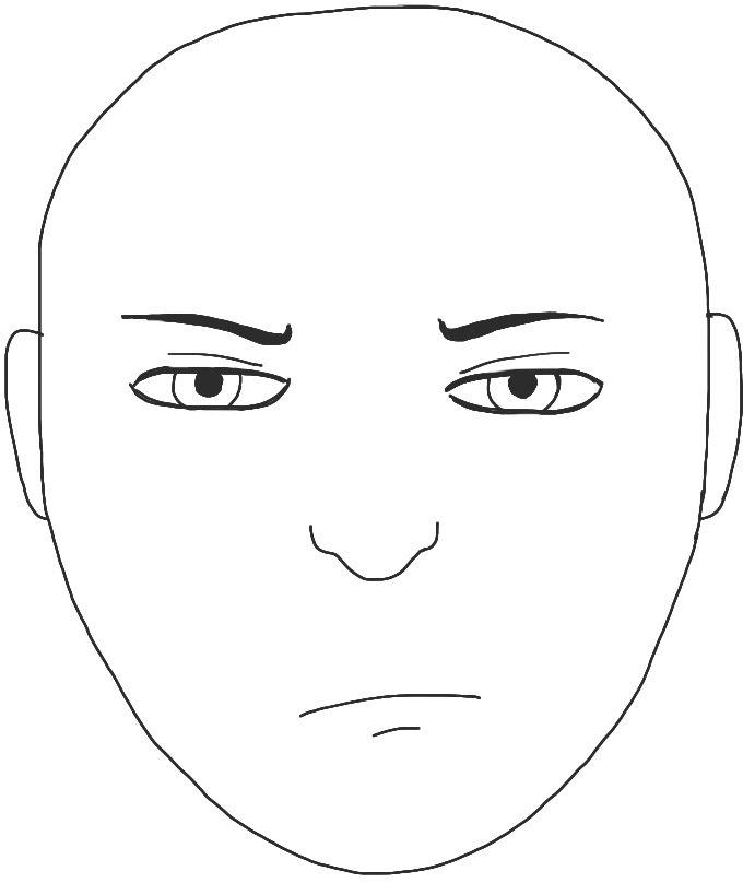
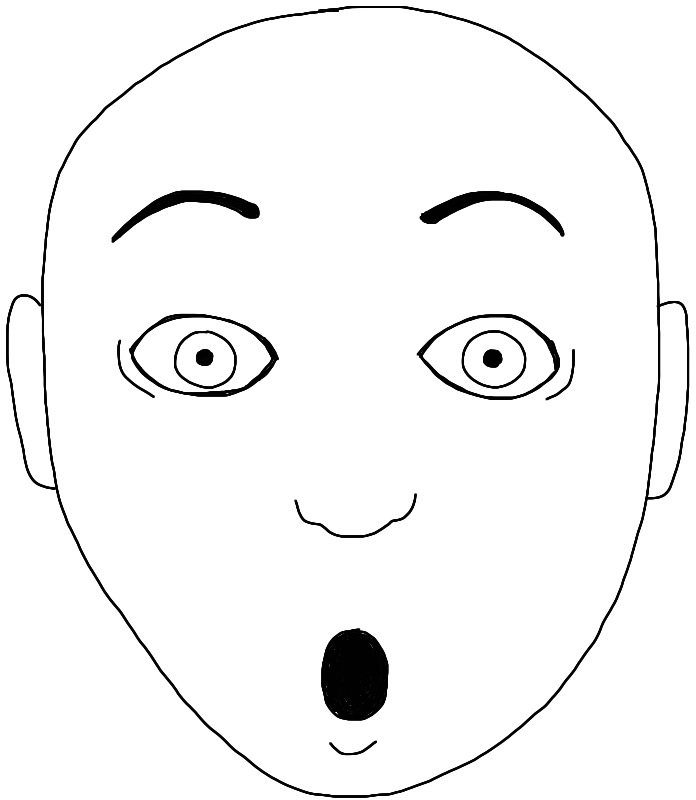
StyleGAN: latent structure
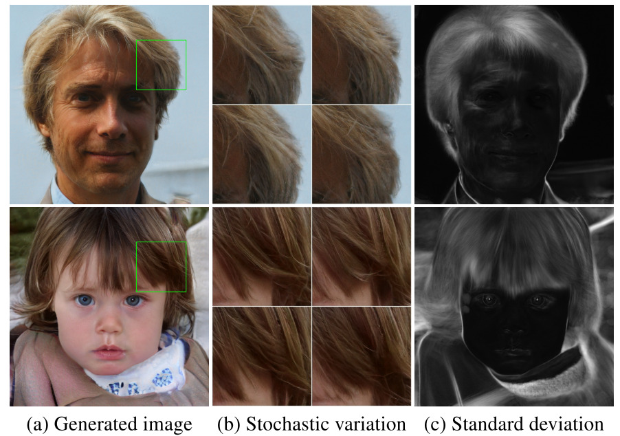
StyleGAN: local noise
![]()
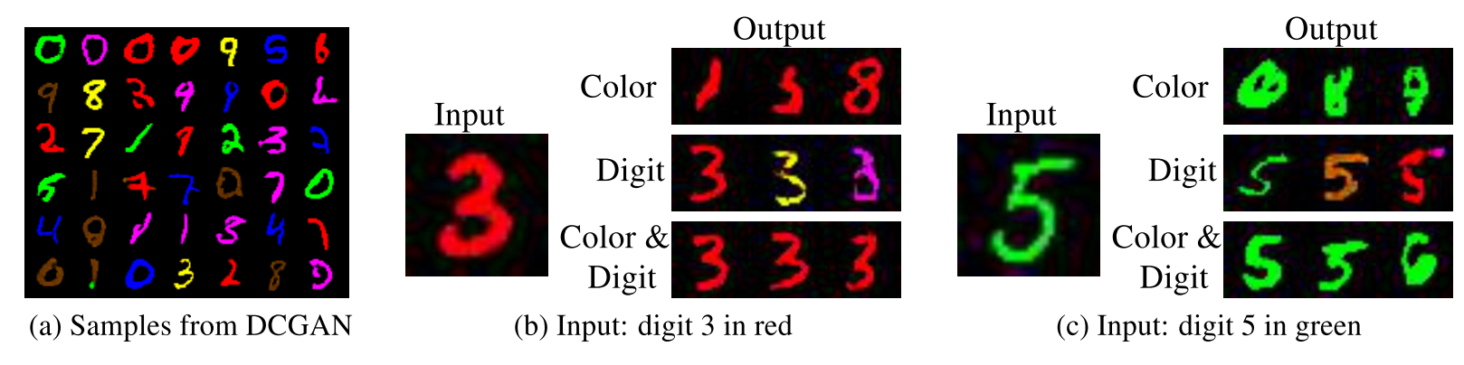
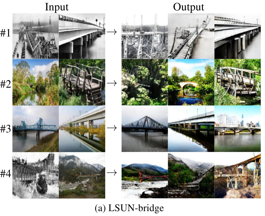
If we want to find “more samples like ”:
![]()
![]()
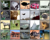
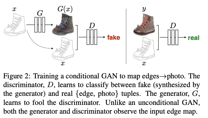
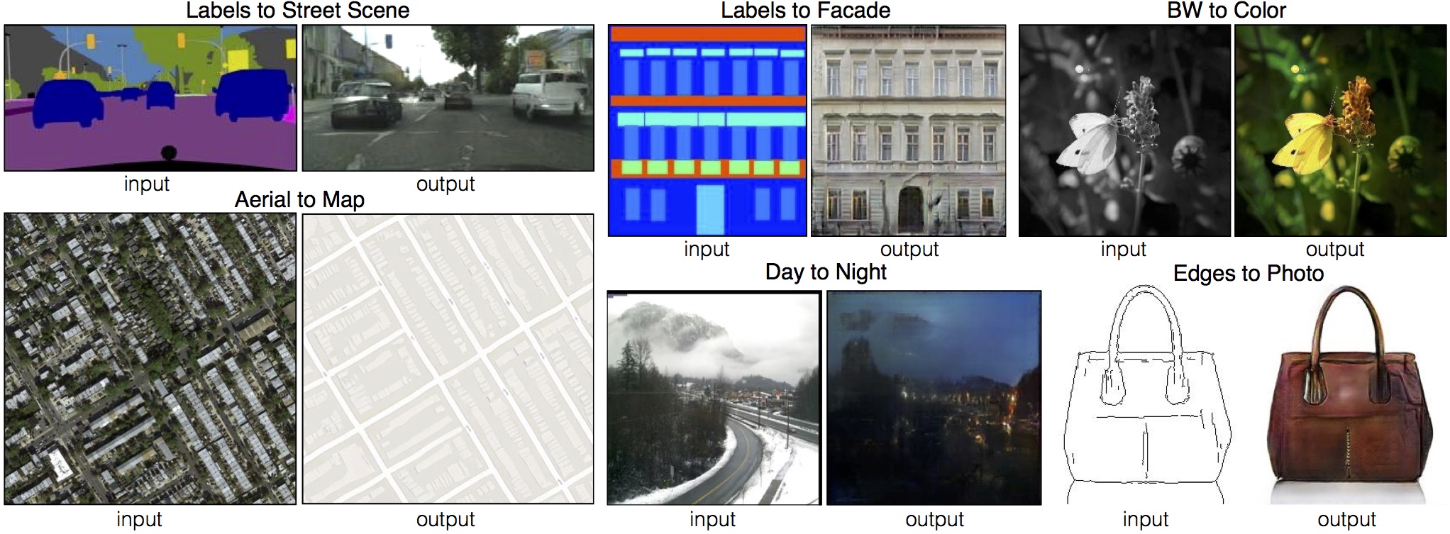
Conditional GANs and BigGAN
- Conditional GANs: [Mirza+ 2014]
- Just add a class label as input to and
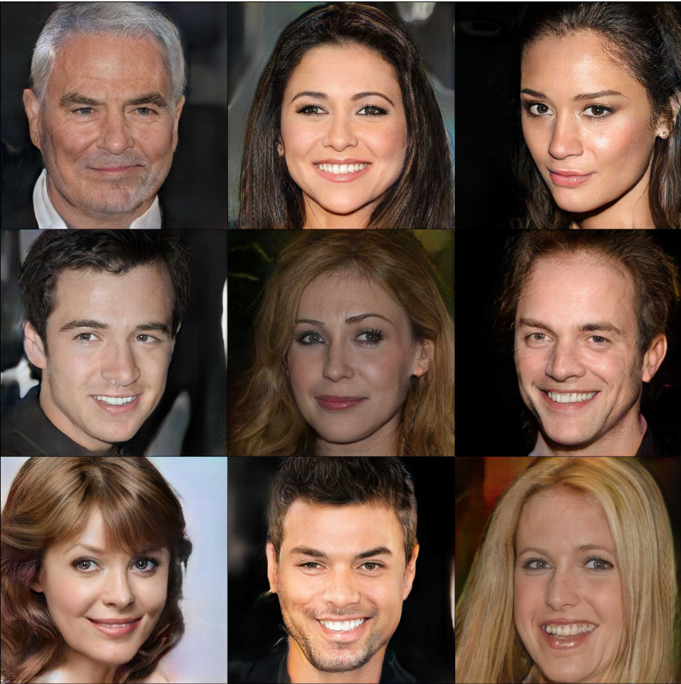
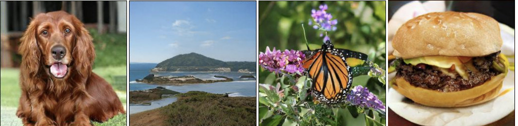
- BigGAN [Brock+ ICLR-19]: a bunch of tricks to make it huge
![]()